It has been a long and winding road, but we have now arrived at the core of each RCT evaluation: the primary effectiveness analysis.
Put simply, the goal of this analysis is to confirm that the intervention has had an effect on the studied population. Yet, this is still very vague. In practice, effectiveness analyses require an unambiguous definition of the effect that should be tested. As we mentioned in the primer article, trial estimands provide a sensible approach to clarify precisely what our effectiveness analysis should estimate. As part of the estimand, we also have to define the outcome based on which intervention effects should be tested. This outcome makes up the primary endpoint of our trial: a specific variable, measured at a specific time, using a specific instrument.
Importantly, the determination of the primary endpoint should not be within the purview of us, the trial analysts. Along with the trial estimand, primary endpoints must be specified a priori, before the actual patient recruitment has begun. If the primary endpoint was not pre-specified, this should be regarded as a serious limitation of the trial. In such instances, there is no way to prove that we have not simply used another outcome than originally intended to “prove” that our intervention works (a questionable research practice known as outcome switching).
In the primer article, we showed that the goal of clinical trials is to estimate the average treatment effect, or ATE. Through randomization, an unbiased estimate of the ATE can be obtained by examining the difference between the means of the intervention and control group (IG and CG) with regard to the primary endpoint \(Y\):
Thus, to show that the intervention had an effect, we have to test if the two group means differ significantly from each other (i.e., that \(|\hat{\mu}_{\text{IG}} - \hat{\mu}_{\text{CG}}| > 0\)). In RCTs, this is most commonly achieved via an analysis of covariance(Montgomery 2017; Dunn and Smyth 2018, vol. 53, chaps. 15.3, 2.9).
4.1.1 Analysis of Covariance
ANCOVAs allow us to examine if two or more groups differ significantly from each other while we control for the influence of one or several covariates. In RCTs, these covariates are patient variables that we recorded before randomization; most commonly the baseline measurement of our primary outcome. In our case, this is depressive symptom severity as measured by the CES-D.
While ANCOVA is sometimes treated as a “special” method for experimental research, it is best understood as a specific type of linear regression. The regression formula can be written down like this:
In this equation, \(Y_{ij}\) is the outcome value of some patient \(j\) in treatment group \(i\); \(\tau_i\) is the estimated effect of some treatment group \(i\) (in our case, \(i\) can either be the Internet-based intervention group or the control group). \(X_{ij}\) is the value of a covariate that was recorded for patient \(j\) in group \(i\). Lastly, \(\epsilon\) represents the residuals of the model. These residuals are assumed to follow a normal distribution with mean zero and variance \(\sigma^2\). This is commonly denoted as \(\epsilon \sim \mathcal{N}(0, \sigma^2)\).
The ANCOVA model above assumes that our treatment variable is effect coded. In our example, this would mean that the treatment variable is either \(-1\) or \(1\), depending on the treatment group (\(1\) = Internet-based intervention, \(-1\) = waitlist control). This ensures that the \(\tau_i\) values sum up to zero:
\[
\sum^{a}_{i=1}\tau_i = 0.
\tag{4.3}\]
Where \(a\) is the number of treatment groups (\(a=2\) in our example). To test the treatment effect, ANCOVAs resort to the principle of variance decomposition, which tells us that the total variation in our data, as measured by the sum of squares (SS), can be partitioned into two components: the variation explained by our model, as well as the unexplained, or residual variation. We can summarize the relationship like this:
The significance of the treatment effect is then tested by comparing the predictor and residual sum of squares while accounting for the (predictor and residual) degrees of freedom. This ratio is assumed to follow an \(F\) distribution, the shape of which is determined by the numerator and denominator degrees of freedom \(\nu_{\textsf{num}}\) and \(\nu_{\textsf{den}}\). They are called like this because one of them, the number of parameters \(p-1\), appears in the numerator of the fraction, while the other, the total sample size \(n - p\), is part of the denominator:
Assuming that the sample size is fixed, high \(F\) values (i.e. a high value of \(\textsf{SS}_{\textsf{Predictor}}\) combined with a low value of \(\textsf{SS}_{\textsf{Residual}}\)) mean that the findings are inconsistent with the null hypothesis of no effect, resulting in a low \(p\)-value.
Most introductory statistics books cover analysis of variance, and much of what we explained here may be nothing new to you. The crucial point to understand here is that Equation 4.5 above explains why we control for covariates in ANCOVAs. To detect a significant treatment effect, we aim for a high \(F\) value; we want the numerator value to be large while minimizing the denominator. This is where covariate adjustment provides a solution: including variables that are predictive of the outcome, such as the baseline symptom severity, allows us to reduce the amount of unexplained variationwithin the treatment and control group. This means that \(\textsf{SS}_{\textsf{Residual}}\) decreases, which in turn automatically leads to a higher \(F\) value.
Thus, the primary rationale for including covariates in ANCOVAs is to enhance our statistical power in detecting treatment effects. With the same sample size, we can get additional power “for free”, just by controlling for factors that explain why patients have lower or higher outcome values within the different treatment groups.
There is a caveat here, however, that we can start to understand if we look closely at Equation 4.5 again. In the equation, we can see that the denominator value is also influenced by the number of parameters \(p\). Thus, controlling for covariates will only increase our power if they are actually predictive of the outcome, and thus reduce the residual variation in our data. If they do not, the only thing that increases is the number of parameters \(p\), and the \(F\)-value actually decreases. Thus, it is important to select covariates carefully. In the next section, we explore this topic a little further.
4.1.2 Covariate Adjustment
Although there is a general agreement that covariate adjustment is a reasonable method in trial analyses, what variables to control for is frequently less clear. Overall, how to best adjust for covariates in RCTs remains an open research question (Permutt 2020; Kahan et al. 2014, 2016; Tackney et al. 2023; Morris et al. 2022). In this section, we want to provide some tentative guidance on how this topic can be approached in practice.
Generally speaking, our goal should be to include covariates that are prognostic of our primary endpoint. However, this does not mean that we should search for “optimal” covariates in our data, for example by examining their correlations with the outcome. Instead, adjustment variables should be pre-specified a priori to rule out that we simply added or removed covariates until the desired results were attained (Assmann et al. 2000).
In the previous section, our ANCOVA model only included one covariate, the baseline measurement of the outcome. However, it is very much possible and often indicated to include several variables. On the other hand, an excessive number of covariates (say 10 or more) should best be avoided. With a large number of covariates, it is likely that many will not explain a sensible amount of variation in our data. Yet they are still counted as additional parameters, thus counteracting our goal to achieve greater power through the adjustment. There are also other reasons that are nicely summed up by a guidance document from the European Medicines Agency (EMA 2015):
“No more than a few covariates should be included in the primary analysis. Even though methods of adjustment, such as analysis of covariance, can theoretically adjust for a large number of covariates it is safer to pre-specify a simple model. […] Results based on such a model are more likely to be numerically stable, the assumptions underpinning the statistical model are easier to validate and generalisability of the results may be improved.”
While these are more general recommendations, there is one case in which baseline adjustment is strictly required. If stratified block randomization was used, it is necessary to adjust for all stratification variables in the analysis (Kahan and Morris 2012). Stratified randomization forces the distribution of the stratification variables to be exactly equal in both groups; random covariate imbalances as they can occur in simple randomization are ruled out a priori. Thus, we have to acknowledge this systematic, non-random factor in our experimental design by including the stratification variables as covariates (Kahan and Morris 2012).
Lastly, we want to emphasize that ANCOVAs, while widely used, are not the only method to adjust for covariates in an effectiveness analysis. In the primer article, we described that trial estimands should be seen as separate from the concrete analysis model; the latter is simply a statistical vehicle that we used to approximate the former. In a similar way, ANCOVAs are not designed to be a “true” parametric model of all the underlying processes that generated our trial data. We use them to obtain an unbiased estimate of the average treatment effect, and including prognostic covariates increases our precision in doing so. Furthermore, if the covariates are truly prognostic of the outcomes, they also allow us to control for chance imbalances that occurred between the randomized groups.
In the ANCOVA model, covariates are included as simple linear terms. In reality, the covariate-outcome relationship may be much more complex than that. There are methods that adjust for the influence of baseline variables in a more sophisticated way; in Section 4.2.3, we will get to know G-computation, which is one of them. However, at least for continuous outcomes, it is debatable if these approaches are truly preferable to a “simple” ANCOVA. Simulation studies have shown that ANCOVA retains its desired properties over a wide variety of scenarios (Wang, Ogburn, and Rosenblum 2019; Egbewale, Lewis, and Sim 2014), and is only surpassed by other methods when there are strong treatment-covariate interactions and non-linear relationships (Tackney et al. 2023). Adding to this the fact that ANCOVAs are fairly easy to specify and interpret makes a strong case to use them as a default method in practice.
A different picture emerges if we want to estimate treatment effects on a binary outcome (e.g. response or remission), and we will cover this issue later in this tutorial.
4.1.3 ANCOVA in Practice
With this theoretical foundation, we now use ANCOVA to examine the treatment effect in our example data. To do this, we first need to make sure that the mitml, purrr and miceadds packages are loaded from the library:
library(mitml)library(purrr)library(miceadds)
Before calculating our treatment effect in the multiply imputed data, let us first have a look at the cases without missings. A complete case analysis (CCA) can serve as a helpful sensitivity analysis because it allows to examine the impact that our imputations had on the results. It is important to stress here that this analysis should only be seen as complementary; typically, it cannot replace the primary effectiveness evaluation conducted in the imputed data. Nevertheless, there are some cases in which a CCA may provide a valid approach even for the main effectiveness evaluation, and not only as a sensitivity analysis. We describe this in greater detail in the infobox at the end of this section.
As described in the previous chapter, ANCOVAs are based on a linear model. Thus, as a first step, we can use the lm function in R to fit a linear regression. As part of our call to lm, a regression formula has to be specified. The box below describes how this is done using R.
Formula Elements in R
Formulas elements in R follow the basic format y ~ 1 + x, where y is the outcome to be predicted, x is the name of the predictor, while 1 symbolizes the intercept (the latter is not mandatory and an intercept will be added automatically if we leave it out). Interactions can be built using an asterisk, for example, x1 * x2. Using the scale function, we can center and scale continuous predictors directly within the formula, for example, y ~ 1 + scale(x).
In our evaluation, we test the intervention’s effect on our primary endpoint (CES-D depressive symptoms at post-test; cesd.1) while controlling for the baseline measurement of the same variable (cesd.0). To conduct a complete case analysis, we can extract the data element from our imp object that we generated using the mice function (see Section 3.2.2). This element contains the original, unimputed trial data. We save the results of the lm function as m.lm. This leads to the following code:
m.lm <-lm(cesd.1~1+ group +scale(cesd.0), data = imp$data)
By plugging the results into the summary function, we can examine the coefficient estimates of our linear regression model:
In the output, we can see that the coefficient of the group variable is \(\hat\beta_{\textsf{group}}\approx\)–6.68. This means that the post-test CES-D scores in the treatment group (group=1) are approximately 7 points lower in the treatment group receiving the internet-based intervention than in the waitlist control group. The control group mean is captured by the intercept: \(\hat{\mu}_{\textsf{CG}}\approx\) 23.05; the mean in the intervention group can therefore be calculated by subtracting the group effect from this value: \(\hat{\mu}_{\textsf{IG}}\) = 23.05 – 6.68 \(\approx\) 16.37.
Looking at the \(t\) and corresponding \(P\) value of our group coefficient, we see that the scores of both groups do indeed differ significantly when controlling for the baseline depressive symptom severity (\(p<\) 0.001). To conduct a “real” analysis of variance and corresponding \(F\) test, we apply the anova function:
anova(m.lm)
Show result
## [...]## Df Sum Sq Mean Sq F value Pr(>F) ## group 1 4361.0 4361.0 59.8613 8.888e-14 ***## scale(cesd.0) 1 1.5 1.5 0.0202 0.8872 ## Residuals 388 28266.4 72.9 ## ---## Signif. codes: 0 ‘***’ 0.001 ‘**’ 0.01 ‘*’ 0.05 ‘.’ 0.1 ‘ ’ 1
In the output, we can see that the test of our treatment effect is significant: \(F_{\text{1,388}}\)=59.86, \(p<\) 0.001. Naturally, these are only the results based on the complete cases. To ascertain that the treatment can be considered effective as per our trial estimand (see Table 2 in the primer article), an analysis based on all randomized participants (i.e., the “intention to treat” sample) is indicated. Thus, we will conduct our main effectiveness evaluation in the data that we imputed under the MAR assumption using MICE.
Complete Case Analysis: Better Than Its Reputation?
Apart from the trivial case in which the number of missings is zero or negligible, there are some plausible scenarios in which a CCA may actually also be valid for our main effectiveness evaluation. Carpenter and Smuk (2021) describe that there are two special cases for which an analysis of imputed data (under the MAR assumption) does not provide any meaningful benefits: (1) when only values in the outcome variable are missing; or (2) when all patients with missing covariate data also have a missing value in the outcome variable. Since baseline measurements are usually more often recorded than follow-ups, both cases are not unrealistic.
However, this reasoning only holds when we have no auxiliary variables in our data that have been observed in patients with missing outcomes, and that are good predictors of missing outcome values. If such auxiliary variables are available, as in our example data set, including them in an imputation model allows to recover additional information that we would not have under a complete case analysis. Many trials include a broad baseline assessment of, e.g., clinical symptoms, demographic variables, risk factors, personality scales, and so forth. If this is the case, an analysis of imputed data sets that incorporate all of this potentially helpful information can be expected to produce better results than a simple complete case analysis.
To begin our analysis of the multiply imputed data, we first convert the imp object we created using mice into an mitml.list object. This type of object contains one imputed data set in each list element and can be used to pool the separate analysis results later on. The mids2mitml.list function can be used to do this conversion. We save the results under the name implist.
implist <-mids2mitml.list(imp)
To confirm that this worked, let us check the class of the newly created object:
class(implist)
Show result
## [1] "mitml.list" "list"
We see that, as intended, the implist object has the class "mitml.list" and "list". Please note that our imputation list always needs to have this class so that the pooling works. If the object does not have the desired class, it is possible to run implist <- as.mitml.list(implist) to reset it.
To run our ANCOVA regression model in each data set, we can use the with function. The first argument specifies the list of imputed data sets, while in the second argument, we provide the same regression formula that we also used in our complete case analysis. Then, use the pipe operator to forward the results to the testEstimates function. This function is part of the mitml package and allows us to obtain the pooled results based on Rubin’s combination rules (see Section 3.3):
with(implist, lm(cesd.1~1+ group + cesd.0)) %>%testEstimates()
In the output, we see that the coefficient of the treatment indicator is \(\hat{\beta}_{\textsf{group}}\approx\) –7.12. This effect is significant: \(t=\) –8.376, \(p<\) 0.001. The output also tells us that the degrees of freedom of this test are \(\nu=\) 770.443. As mentioned before, this somewhat “odd” number is a consequence of the formula that is applied to derive the degrees of freedom in multiply imputed data (see Section 3.3.2).
In the RIV and FMI columns, we are presented with the relative increase in variance due to non-response and fraction of missing information for each coefficient estimate. For our group term, these values are \(r_{\beta}=\) 0.337 and \(\gamma_{\beta}=\) 0.254, respectively.
The FMI value is typically a better indicator to gauge the actual “costs” that missingness had on our estimates than, say, the percentage of missing values in a variable (Madley-Dowd et al. 2019). In our example, despite the auxiliary variables in our imputation model, approximately 25.4% of the variation in our estimates is due to the uncertainty of our imputations; the \(r\) value tells us that this represents an 33.7% increase in variance. This loss of information and the resulting increase in the variance of our estimate could have been avoided had the data been completely recorded, and parts of it could have been avoided had we been able to build an even better imputation model using further auxiliary variables.
Another thing to note about the output is its last line. This tells us that an unadjusted hypothesis test “as appropriate in larger samples” was conducted. By default, testEstimates returns results based on the large-sample formula, which assumes that the complete sample degrees of freedom are infinitely large (see Section 3.3). Our example trial included \(N =\) 546 participants, which means that this method may be roughly appropriate. Nevertheless, let us also check if the results change dramatically if the small sample formula is applied. To do this, we first have to calculate the complete-sample degrees of freedom, \(\nu_{\textsf{com}}\):
# df.com is defined as sample size minus the number of parameters:df.com <-nrow(imp$data) -length(coef(m.lm))
Then, we can provide this value within our call to testEstimates, which will automatically apply the alternative formula:
with(implist, lm(cesd.1~1+ group + cesd.0)) %>%testEstimates(df.com = df.com)
Show result
## [...]## Estimate Std.Error t.value df P(>|t|) RIV FMI ## (Intercept) 23.453 1.642 14.287 321.113 0.000 0.248 0.204 ## group -7.124 0.851 -8.376 265.274 0.000 0.337 0.258 ## cesd.0 -0.004 0.059 -0.072 275.845 0.943 0.318 0.247 ## ## Hypothesis test adjusted for small samples with df=[543]## complete-data degrees of freedom.
We see that the degrees of freedom for our group coefficient are now 265.274, considerably smaller than the 770.443 from before. Apart from that, the results are almost identical.
In the last step, we run the “classic” \(F\)-test conducted as part of an ANCOVA. This means that we first have to run an analysis of variance using the anova function, and then extract the \(F\) value for our treatment effect. Since we are working with multiply imputed data now, we have to employ the map to perform this operation in all list elements simultaneously. We use the map_dbl function here, which returns a vector of \(F\) values from each data set that we save as Fvalues.
with(implist, lm(cesd.1~1+ group + cesd.0)) %>%map_dbl(~anova(.)$`F value`[1]) -> Fvalues
As described before (see Section 3.3), it is not possible to pool test statistics by taking their mean; we have to apply specialized formulas instead. In our case, we can use the micombine.F function in the mitml package to aggregate the \(F\) values correctly:
micombine.F(Fvalues, df1=1)
Show result
## Combination of Chi Square Statistics for Multiply Imputed Data## Using 50 Imputed Data Sets## F(1, 722.34)=69.384 p=0
The result is \(F_{\text{1,722.34}}=\) 69.38, which is significant: \(p<\) 0.001. Thus, we can conclude that the internet-based intervention was effective in this trial.
However, we also want to check the robustness of this effect by conducting a sensitivity analysis in data sets imputed using the “jump-to-reference” method. In Section 3.2.3, we saved the imputed data in an object we called imp.j2r. This object can also be transformed into a list of data sets using the mids2mitm.list function.
However, the resulting data still needs an additional preparation step. To run the imputation model, we had to convert our data into the long format. Now, to run the same type of analysis as in the main effectiveness evaluation, wide-format data is required. Thus, we use the pivot_wider function to return the imputed data sets back to their original format. Since this has to be done in all sets simultaneously, we plug the operation into the map function. Please note that the pivot_wider function needs to be loaded for the code below to work.
If prepared in the same way as in this example, this code should be usable for all kinds of trial data. It may only be necessary to adapt the values of time accordingly. In our trial, assessments were obtained after 7 and 12 weeks; of course, this may differ from study to study, meaning that the code has to be changed correspondingly.
If we check the class of the resulting implist.j2r element, we see the issue we mentioned further above: the object class has now changed from mitml.list to a simple list.
class(implist.j2r)
Show result
## [1] "list"
This means that the testEstimates function we use to pool the parameter estimates will not work. To solve this, we have to reconvert the data using as.mitml.list:
implist.j2r <-as.mitml.list(implist.j2r)
Then, we are ready to apply the same covariate-adjusted linear model we used for the main effectiveness analysis:
with(implist.j2r, lm(cesd.1~1+ group + cesd.0)) %>%testEstimates()
We see that, like in the main analysis, the treatment coefficient is significant: \(t_{\text{1328.702}}=\) –5.599, \(p<\) 0.001. Notably, the imputation uncertainty is lower in the J2R-imputed data, as indicated by an FMI value of \(\gamma_\beta=\) 0.193. However, we also see that the reference-based imputation leads to a more conservative estimate of the treatment effect: \(\hat{\beta}_{\textsf{group}}\approx\) –4.73, compared to the value of –7.12 we found in the data we imputed using mice.
As we have learned, jump-to-reference imputation is based on the conservative (but not impossible) assumption that all patients behave exactly like the control group once they are lost to follow-up. Given that the number of missings at post-test is substantial, we see that such an assumption almost halves the treatment estimate we obtain when assuming MAR. However, we also see that this effect is still significant, which provides further evidence that the effect detected in the main analysis is indeed robust. In practice, we would also conduct an \(F\)-test for the J2R-imputed data using the same code we used for the main analysis. We omit this step here.
One-Sided Testing: A Good Idea?
In the analyses above, we used two-sided tests to confirm that our treatment was effective. These two-sided tests are the default returned by most implementations in R. A two-sided test is based on the null hypothesis of no effect, \(\mu_1 - \mu_2=\) 0, which allows testing for both positive treatment effects (meaning that the intervention was beneficial) as well as negative effects.
One could argue that in RCTs, our hypotheses are not really two-sided. We want to know if the evaluated treatment is better than the control group, not if it is better or worse. This fits better with a one-sided test, which also happens to give us greater power than two-sided testing. Some have argued along these lines to propose that one-sided testing is preferable, at least in many contexts (Knottnerus and Bouter 2001; Owen 2007).
While there is some controversy surrounding the question of one- vs. two-sided testing, the general consensus in the medical literature seems to be that two-sided testing should be used as the default approach (Lydersen 2021). There are good reasons for this: if a one-sided test is conducted, we cannot make any statements on potential negative effects that the intervention may have had, even if our data (e.g. the mean difference between two groups) indicates that this is a possibility (Moyé́ and Tita 2002). Effects in the opposite direction may not be likely, but they are possible; mental health treatments can indeed be harmful (McKay and Jensen-Doss 2021; Lilienfeld 2007; Hengartner 2017), and it is difficult, if not impossible, to rule out a priori that this will not be the case in our trial.
Obviously, no matter if a one- or two-sided testing strategy is used, this must be pre-specified in the analysis plan. Otherwise, we may be tempted to switch from a two- to a one-sided testing strategy because our treatment effect would not be significant otherwise. It goes without saying that this would constitute a highly questionable research practice.
4.1.4 Calculating the Standardized Mean Difference
In the previous chapter, we demonstrated the effectiveness of our intervention. Now, we want to quantify this effect using a measure that is interpretable beyond the specific context of this trial. This is typically achieved by calculating effect sizes.
The term “effect size” is not clearly defined. Some people think of effect sizes as standardized mean differences (SMDs), also known as Cohen’s \(d\), while others prefer a broader definition. The “narrow” definition may be difficult to uphold, since correlations, odds ratios, \(Z\) values, etc., can also express the direction and strength of an effect, and can even be partly transformed into each other (Harrer et al. 2021, chap. 3.1).
Within RCT analyses, effect sizes are used to quantify the size of the treatment effect, and make it comparable to similar studies. For continuous outcomes, the most commonly used effect size measure is the standardized mean difference, the true value \(\theta\) of which is defined as:
where \(\mu_{\textsf{IG}}\) and \(\mu_{\textsf{CG}}\) are the true means of the intervention and control group, and \(\sigma\) is the true standard deviation of the outcome in the population. Notably, none of these three quantities can be directly observed; we can only estimate them from our trial data. This is typically done by replacing the \(\mu\)’s with the intervention and control group means \(\bar Y_{\textsf{IG}}\) and \(\bar Y_{\textsf{CG}}\), and \(\sigma\) with the pooled standard deviation \(s_{\textsf{pooled}}\) of our outcome \(Y\) in both groups. This leads to the “classic” formula for what is commonly known as Cohen’s\(d\):
Notably, \(s_{\textsf{pooled}}\) can also be replaced by other, external estimates of \(\sigma\) if they are available. This may be particularly helpful when our trial sample is small, or when there are other reasons to believe that \(s_{\textsf{pooled}}\) is a bad estimator of the population standard deviation. Sometimes, the control group standard deviation alone is also used to standardize the mean difference, for example when there is more than one intervention group. This, however, leads to a different effect size metric known as Glass’ \(\Delta\).
Equation 4.7 above is typically used to calculate the between-group Cohen’s \(d\) in clinical trials and meta-analyses. In practice, a greater challenge is the construction of valid confidence intervals around this point estimate. For many effect sizes, including \(d\), there are closed-form equations to calculate the sampling variance, which is required to determine the confidence intervals. However, if we use these formulas for effect sizes derived from multiply imputed data, we neglect that our estimates are also additionally affected by imputation uncertainty. This would lead to anti-conservative results; that is, confidence intervals that are too narrow.
A more elegant way to calculate effect sizes is to derive them from the linear covariate-adjusted model we used to estimate the treatment effect. In our model, we estimate \(\beta_{\textsf{treat}}\), which can be interpreted as the mean difference in outcomes between the two groups: \(\hat\beta_{\textsf{treat}} = \widehat{\text{ATE}} = \hat\mu_{\textsf{IG}} - \hat\mu_{\textsf{CG}}\). Covariate adjustment within the model ideally means that our estimate of this treatment effect becomes more precise and that we control for random imbalances in prognostically relevant baseline variables. Using Rubin’s rules, we can also obtain valid confidence intervals around our parameter estimate that incorporate our imputation uncertainty.
Therefore, we can calculate an estimate of the true effect size, as well as its lower and upper confidence limit, if we standardize \(\hat\beta_{\textsf{treat}}\) by the pooled standard deviation:
Time to illustrate this in practice. First, we need to calculate \(s_{\textsf{pooled}}\). We can do this by extracting the intervention and control group standard deviation from each imputed data set in implist, and then taking the mean value. Then, we use the formula in Equation 4.7 to obtain the pooled value.
Calculate mean SD for both groups across imputed data sets.
2
Define sample size in both groups.
3
Calculate pooled standard deviation.
Show result
## [1] 8.585904
We see that \(s_{\textsf{pooled}}\approx\) 8.586. We can now use this value to standardize the mean difference estimated by the coefficient of group. A convenient way to do this is to include the “AsIs” function I directly in the model formula. Specifically, we are writing I(cesd.1/8.586) in the outcome part of the formula to indicate that the coefficients should be divided by the pooled standard deviation we just calculated. For the main effectiveness analysis, this leads to the following code:
(m.es <-with(implist, lm(I(cesd.1/8.586) ~1+ group + cesd.0)) %>%testEstimates())
In the output, we see that the coefficient of our group term is now –0.83, which can be directly interpreted as the value of Cohen’s \(d\). To create a confidence interval around the effect, we can plug the model into the confint function:
Thus, we see that the effect size, based on the main effectiveness analysis, is \(d=\) –0.83, with the 95% confidence interval ranging from –0.64 to –1.02.
Next, we use the same approach to calculate the effect size for our complete case analysis:
(m.es.cca <-lm(I(cesd.1/8.586) ~1+ group + cesd.0, data = imp$data))confint(m.es.cca)
This results in a roughly comparable estimate of \(d=\) –0.78 (95%CI: –0.58 to –0.98). Lastly, we can also calculate the effect size based on our reference-based imputation analysis:
(m.es.j2r <-with(implist.j2r, lm(I(cesd.1/8.586) ~1+ group + cesd.0)) %>%testEstimates())confint(m.es.j2r)
As we discussed before, the effect here is considerably lower, with \(d=\) –0.55 (95%CI: –0.36 to –0.74).
Interpretation of Cohen’s \(d\)
Values of \(d\) are often interpreted in reference to the “rule of thumb” by Cohen (1988), which states that \(d=\) 0.2, 0.5, and 0.8 represent small, moderate, and large effects, respectively. A better approach is to compare the effect sizes in our trial to other, similar studies; or to established, field-specific reference values.
For depression treatments, for example, it has been found that the minimally important difference that patients would still recognize as beneficial is \(d=\) –0.24 (Cuijpers et al. 2014). All the effect estimates we obtained in our example analyses (\(d=\) –0.55 to –0.83) are above this threshold, suggesting that the effects of our intervention can be considered clinically meaningful.
4.2 Binary Endpoints
In our example trial, the primary endpoint was depressive symptom severity, which can be intuitively expressed on a continuous scale. In other trials, the primary endpoint may be binary, that is, based on a condition that is either met or not met. A natural example are trials in which the primary outcome is patients’ diagnostic status at some follow-up assessment (especially in trials in which all patients fulfilled the diagnostic criteria at baseline).
We may also be interested in how a treatment affects individuals’ diagnostic status over time. This can be done by comparing the incidence rates of different groups; or, if many assessments over time are available, via a survival analysis. The latter is frequently used in prevention trials to examine if some treatment reduces the hazard of developing a mental disorder within the examined time frame. Survival analysis is a multi-faceted topic that we do cover here. Luckily, however, there are helpful resources that detail how such analyses can be implemented using R (Moore 2016).
In other cases, binary outcomes are derived from endpoints that were originally measured on a continuous scale. This is typically done to transform outcomes into results that can be more easily interpreted by clinicians and laypeople. We achieve this by determining the number of patients who experienced some form of reliable or clinically significant change during the study period, and if these numbers differ significantly between groups. In the following section, we will discuss ways to determine such binary metrics of change and showcase how to calculate the most commonly used one. This will also provide us with a binary endpoint that we will analyze afterwards.
Before we start, we want to issue a cautionary note concerning the “derived” binary outcome measures that we will be calculating next. From a statistical perspective, pigeonholing a continuous outcome into simple yes/no metrics is a questionable practice that is known as dichotomania among trial statisticians (Senn 2005). Dichotomizing continuous endpoints means that we actually lose a lot of outcome information, and it typically forces us to put patients into completely distinct categories, even if they hardly differ in their outcomes. In the context of our example trial, the following analyses should only be seen as supplementary to the main evaluation we conducted in the previous chapter.
4.2.1 Reliable Change & Minimal Clinically Important Differences
A widely used method to determine which patients improved during the study period is the reliable change index, or RCI (Jacobson and Truax 1992). This metric is particularly common in clinical psychology and often found in psychotherapy trials. The reasoning behind the RCI is that, if we find a difference between some person \(i\)’s score at baseline and some later assessment, it is unclear if this represents real symptom change, or simply some random variation attributable to measurement error. Thus, we need a measure that allows us to gauge if some pre-post difference \(Y_{1,i}-Y_{0,i}\) in the outcome \(Y\) truly represents reliable change. The RCI allows us to do this by standardizing the “raw” score difference by an estimated standard error of measurement, \(s_{\textsf{diff}}\):
In this formula, \(s_{0}\) is the baseline standard deviation of \(Y\), and \(r_{YY}\) is the test-retest reliability of our instrument. This reliability coefficient has to be determined from previous literature. Typically, estimates of validation studies in similar populations are used for this.
The calculated RCI values of each participant can then be employed to identify those who have achieved reliable change. Similar to \(Z\)-scores, we assume that the RCI values follow a standard normal distribution with a critical value of 1.96. Thus, if RCI \(\leq\) –1.96, we conclude that a person reliably improved (assuming lower values indicate better outcomes). If RCI \(\geq\) 1.96, a person experienced reliable deterioration. All difference scores in between are counted as unchanged:
We have implemented Equation 4.10 above into a function that can be used to calculate RCIs using R. This function is not pre-installed, so we have to let R “learn” it by copying and pasting the code below into the console, and then hitting Enter.
As we have mentioned, the RCI formula requires us to provide an estimate of the test-retest reliability of our instrument. In our example, we use a value of \(r_{YY}=0.85\), which has been calculated in a previous study that validated the CES-D.
ryy <-0.85
Before we use the rci function in practice, let us first determine the value of \(s_{\textsf{diff}}\). Using map, we calculate the value in each imputed data set and then take the mean. Please note that this is not technically necessary in our example trial, in which all baseline values are recorded; but the code below may come in handy if this is not the case. We save the result as s_diff.
We see that in our trial, assuming \(r_{YY}=\) 0.85, the standard error of measurement is \(s_{\textsf{diff}}=\) 3.905. Thus, we conclude that a reliable symptom change occurred if the change between baseline and post-test is greater than 1.96 \(\times\) 3.905 \(=\) 7.654 points.
Next, we calculate for each of our patients, if they experienced reliable improvement or deterioration based on the RCI. We again have to do this in all imputed data sets, for which we use map again. In the supplied function, we use the rci function to create a new variable in which the exact RCI value of each person is stored. Then, we use the ifelse function to determine if the RCI value is above 1.96 or below –1.96. This results in binary indicator variables (i.e., a variable that is either 1 or 0) for reliable improvement (ri) and deterioration (rd).
Create binary indicator for reliable improvement & deterioration.
Each element in implist now contains three new variables containing the RCI value, as well as the reliable improvement and deterioration indicator for each patient. For now, the outcome we are most interested in is reliable improvement. Thus, we now summarize the number of individuals with reliable improvement in both treatment groups and aggregate the values across all imputation sets. This can be achieved using the code below. We save the result as table.ri:
This leaves us with a 2 \(\times\) 2 table, with the rows indicating the group (0 = control, 1 = intervention), and the columns indicating the reliable improvement status (0 = not improved, 1 = reliably improved). We see that considerably more individuals in the intervention group (\(n=\) 166) experienced a reliable improvement than in the control group (\(n\) =100), although we do not know yet if this is statistically significant.
Based on these cell counts, we can also derive another metric that is commonly calculated in trials: the number needed to treat, or NNT. This treatment effect measure is often used because it is easier to understand by clinicians and other stakeholders1. NNTs indicate, based on the present evidence, the number of individuals that needs to be treated with the intervention to cause one additional positive event in the studied population. In our example, this would be one additional case of reliable improvement. Depending on the nature of the outcome, NNTs can also be interpreted as the number of patients we need to treat to prevent on additional negative outcome (e.g. symptom deterioration).
NNTs not only depend on the treatment effect but also on how common or uncommon an event is in general. Even if a treatment is very effective, if the event under study is extremely rare, this still means that we have to treat a lot of patients to cause or prevent one additional case, given that most people would not have experienced the event anyway. Naturally, this leads to a much higher NNT than when the event is very common.
NNTs can be calculated as the inverse of the absolute risk reduction, or ARR. The ARR itself is determined by subtracting the event rate in the control group \(p_{e_{\textsf{control}}}\) from the event rate in the intervention group \(p_{e_{\textsf{treat}}}\):
Calculate proportion of reliable improvement cases.
3
Calculate NNT (inverse risk reduction).
Show result
## [1] 4.136364
We see that the result is NNT \(\approx\) 4.14. Rounding this value up, we can say that five patients need to receive the Internet-based intervention to generate one additional case of reliable improvement. While this may seem high at first glance, this is actually quite a low value for a mental health intervention. In preventive contexts, it is not unusual to find NNTs of 20 or higher.
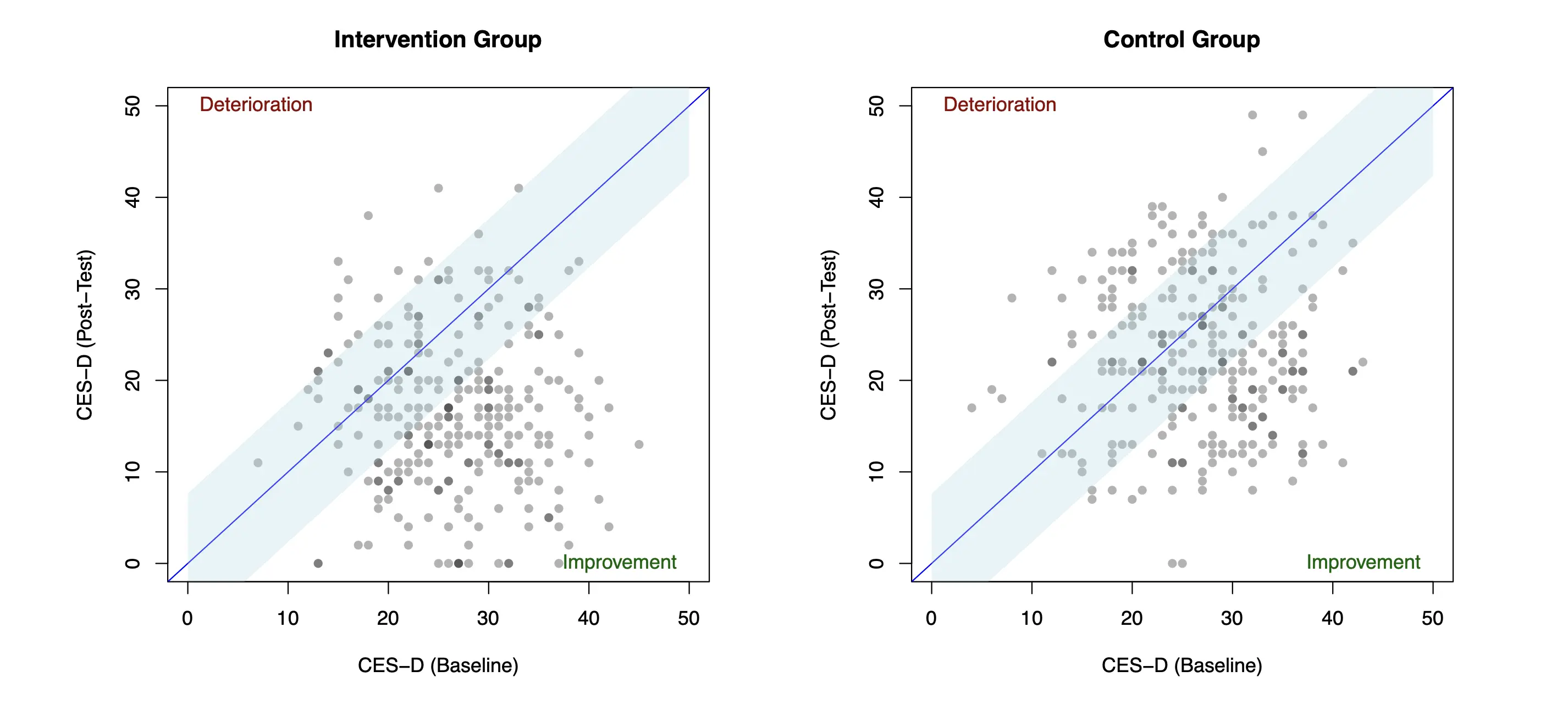
Lastly, we can also visualize the reliable change patterns in our data. For simplicity, we will only plot the data of one imputation set here, and we will choose the first one. To produce a plot for each group, we generate two separate data sets dat.plt.ig and dat.plt.cg.
Making plots in R can be tricky, especially for beginners. However, it is not crucial to understand everything about the code we use below. The syntax can also be adapted by changing the name of the cesd.0 and cesd.1 variable to the relevant outcome measured at baseline and post-test in your particular trial. The same is also true for the axis labels provided in the xlab and ylab argument.
The graphs show, for each participant, the baseline CES-D values on the x-axis, and the post-test values on the y-axis. When there is no difference between the pre- and post-test scores, individual points will end up exactly on the diagonal. The light blue bands represent score changes that we are willing to attribute to measurement error, meaning that all points in this region are categorized as unchanged. Beyond the blue band, points in the lower triangle represent cases with reliable improvement, and points in the upper triangle are those with reliable deterioration. As we can see, the number of reliably improved patients in the lower triangle is considerably higher in the intervention compared to the control group.
The Perils of Standardization: Some Problems with the RCI
Although widely used in mental health research, the RCI has certain limitations that we should acknowledge (Wise 2004; McAleavey 2021). If we go back to Equation 4.10 we see that, besides the raw change score, the RCI depends on two variables: the reliability coefficient \(r_{YY}\), and the in-sample standard deviation at baseline \(s_{0}\).
Selecting a good value of \(r_{YY}\) can be challenging because it has to be determined from previous literature. It is often unclear if the validation sample is representative of the type of patients in our trial. It also leaves us with many researcher degrees of freedom: the size of \(s_{\textsf{diff}}\) depends heavily on the reliability coefficient, so we may be tempted to always select the highest value we find in the literature to make sure that the number of “reliably” improved individuals is as large as possible. Furthermore, it is important to remember that only the test-retest reliability can be used to calculate RCIs. Often, measures like Cronbach’s \(\alpha\) are used instead, which can lead to wildly incorrect results.
This ambiguity also means that the comparability of reliable improvement rates across different trials may be limited. This is further exacerbated by the second variable, \(s_{0}\), which can vary considerably between trials, even when the same instrument was used in similar populations. We use the RCI to determine if a specific patient in our trial has reliably improved or deteriorated. It is odd that this individual response measure depends on the variability of other people’s scores in the trial, but this is exactly what happens if we use the RCI.
Imagine the following scenario: we have two patients with exactly the same pre- and post-test scores, but one happened to be part of a trial with few inclusion criteria and large \(s_{0}\), while the other was included in a trial with very strict inclusion criteria, and thus a very low baseline standard deviation. Both patients experience exactly the same symptom decrease, but in the first trial we would likely regard this as “unchanged” (because \(s_{0}\) is large) whereas, in the second trial, we would consider this change to be a reliable improvement. From a patient perspective, it is illogical that my improvement may depend on the specific trial is was lucky or unlucky enough to get assigned to.
The RCI performs a type of “standardization”, but since this depends on quantities calculated within our sample, our results may often be less comparable than we think they are. In a famous paper, Cohen (1994) describes that this issue also pertains to all kinds of standardized effect measures, including Cohen’s \(d\).
We have now determined the reliable improvement and deterioration status for each of our patients. The ri variable we calculated in this chapter will be reused in the next section, where we describe how to run an effectiveness analysis based on binary outcome data.
It is important to stress that the RCI is by no means the only measure we can calculate from continuous outcome data. There is a completely different strain of metrics revolving around the concept of “clinically significant” (CS) change, which is measured by falling below a practically or clinically relevant cut-off. Such cut-offs are available for many commonly used symptom questionnaires in mental health research, for example, the PHQ-9 (Manea, Gilbody, and McMillan 2012), GAD-7 (Spitzer et al. 2006), or CES-D (Vilagut et al. 2016).
The problem with these cut-offs is that they do not account for baseline symptom severity. Say, for example, that a score of \(Y\leq\) 10 on an instrument represents symptoms that are not clinically relevant anymore. If a person changes from \(Y_0=\) 11 to \(Y_1=\) 10, we would hardly consider this an important change, but the person would still be considered to have experienced clinically significant change. Thus, the RCI and CS measures are often combined to obtain rates of reliable and clinically significant improvement (RCSI), where patients have to show both reliable improvement and score below a certain cut-off.
We may also calculate improvement rates using minimally important differences, or MIDs. Typically, MIDs are minimum raw change scores for a specific outcome that a patient needs to surpass for it to be considered meaningful from a patient’s perspective. A plethora of MIDs have been developed for various mental health questionnaires, but such validation studies unfortunately often differ in their examined populations, methodology, and overall quality (Devji, Carrasco-Labra, and Guyatt 2021). If MIDs are to be used, it is advisable to search for reference values obtained using so-called anchor-based methods. These approaches determine minimally important changes based on an external “anchor”; for example, a clinician or self-report assessment if a patient feels “slightly better” after the treatment.
Yet another response metric is the effective dose 50, or ED50 (Bauer-Staeb et al. 2021), which encodes a 50% probability of patients “feeling better” given their initial baseline severity. This measure is commonly used in pharmacological trials. It is less common in behavioral mental health studies, although it is also applicable in these contexts. In R, this approach can be implemented using the ed50 package (Gan, Yang, and Mei 2019).
4.2.2 Generalized Linear Models
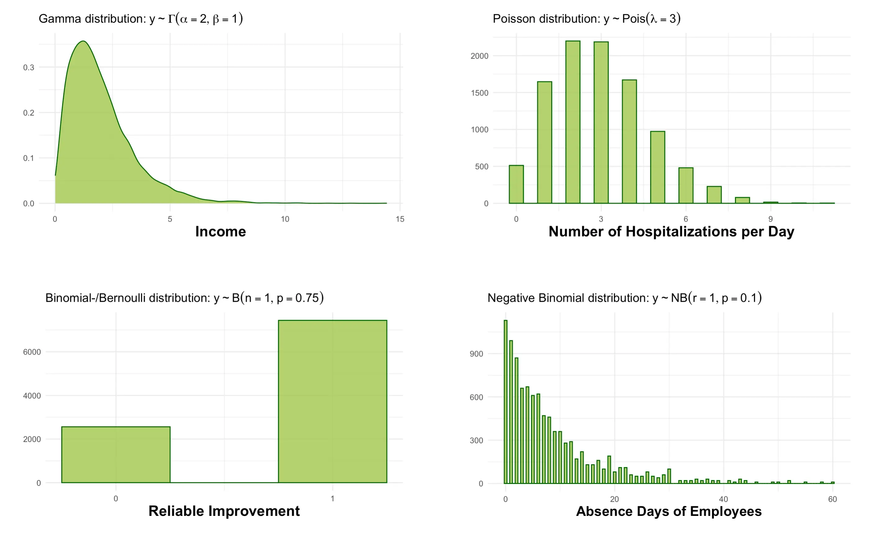
In the previous chapter, we learned how to evaluate treatment effects using ANCOVA (i.e., a covariate-adjusted linear model), which is suitable when our primary endpoint is continuous. However, there are many realistic scenarios in which we cannot assume that our outcome is continuous, and approximately follows a normal distribution. A few examples are provided in the graphic below.
Reliable improvement, which we calculated in the previous section, is a prominent example. We assume that improvement is a binary outcome, where the proportion of improvement and non-improvement is determined by a Bernoulli distribution with an unknown parameter \(p\). To test our treatment effect, we need a linear model that allows to accommodate this alternate distributional assumption for our endpoint. This is where generalized linear models(GLM, Dunn and Smyth 2018, vol. 53, chap. 5) provide a solution.
As it says in the name, GLMs are a generalization of the linear model to the entire exponential dispersion model (EDM) family. A few distributions in this family are displayed in the figure above. In practice, GLMs are frequently used to model count and event data, or other dichotomous outcomes. Computationally, there is a difference between the “standard” linear model and GLMs: the former can be derived directly with ordinary least squares (OLS); that is, using basic matrix algebra. For GLMs, coefficients need to be determined iteratively using maximum likelihood estimation (MLE). This means that the latter are more computationally intensive. Yet, this is typically barely noticeable in R in terms of computation time.
GLMs consist of two components: a linear predictor \(\eta_i\), and a link function\(g(\cdot)\):
Where \(\mathbf{X}\) stands for all the variables we want to include in our linear model, in our case the treatment indicator and covariates. In this context, the inverse of the link function “translates” values of the linear predictor back into the format of the outcome variable: \(g^{-1}(\eta_i) = \mu_i\); \(\mu = E(Y_i)\).
The \(o_i\) term in Equation 4.12 above represents an offset, which is often used in Poisson and negative binomial models. Offsets are a priori known values for which no parameter estimation is necessary. They are frequently used to model the time of exposure \(E\) in the analysis of certain clinically relevant events. Say, for example, that we conducted a trial in aftercare in which we recorded if patients relapsed, but that the follow-up times differed slightly between patients. In this case, patients differed in the time in which they were exposed to the risk of relapse, and this exposure time \(E\) should be accounted for in our model.
Data like this are typically fitted using a Poisson model in which \(E\) serves as the offset. This offset is used to “standardize” the resulting response by the exposure time:
It is not essential to understand everything about the formula above. The crucial message is that offsets are a helpful way to incorporate the effect of time into an analysis model. In R, we could fit a Poisson model with exposure time E, treatment indicator trt, covariate x and outcome y like this:
glm(y ~ trt + x +offset(log(E)), data = data, link = poisson)
The code above already displays the core arguments we need when fitting a GLM using R. In the first argument, we specify the model formula, as we have for our ANCOVA model. Here, we additionally use the offset function to include an offset term. The special argument in the glm function is link. Here, we specify the link function that corresponds with the assumed distribution of our outcome variable.
In Table 4.2 below, we summarize some of the main link functions used in GLMs, and how they can be implemented in R. In Section 4.1.3, we already described that the group coefficient in linear models can be elegantly expressed as the estimated mean difference in our trial and that we can derive the treatment effect size expressed as Cohen’s \(d\) from this value. GLMs follow a similar logic if we use the antilog (i.e., the reverse logarithm) on the estimated treatment coefficient \(\beta_{\textsf{treat}}\). In R, the exp function can be used to take the antilog.
The table shows the effect size metric that the resulting value can be interpreted as, for each respective link function. We see, for example, that \(\beta_{\textsf{treat}}\) gives us the odds ratio (OR) for models with a binomial logit-link (more commonly known as logistic regression). For Poisson models, taking the antilog leads to an estimate of the incidence rate ratio (IRR).
As a next step, we will use a GLM to test the effect of our Internet-based intervention on reliable improvement. For now, let us employ the same formula we used in the ANCOVA model in Section 4.1.3, where the outcome is regressed on the treatment indicator (treat) while adjusting for baseline symptom severity (cesd.0) as a covariate. Naturally, the outcome in our formula is now different: we want to examine effects on reliable improvement as captured by the variable ri in our data, which can either be 1 (improved) or 0 (not improved).
With our outcome ri being binary and measured at the same time point, the binomial logit is a natural choice for our link function. This means that we can fit a logistic regression model to our data. Logistic regression is the most widely used method for binary outcome data because it has desirable computational properties. As we learned, GLMs need to be fitted using an iterative process, and logistic regression models usually arrive at the optimal solution rapidly and without errors. This is one of the great advantages of logistic regression compared to, say, log-binomial models, where the computation is considerably more challenging, and often fails (Williamson, Eliasziw, and Fick 2013).
Thus, in our call to glm, we set the link argument to binomial("logit"). As before, we use the with and testEstimates functions in mitml to obtain a pooled result from the multiply imputed data. The final code looks like this:
implist <-as.mitml.list(implist)with(implist, glm(ri ~ group +scale(cesd.0), family =binomial("logit"))) %>%testEstimates() -> m.glm; m.glm
The structure of the output is identical to the one of our ANCOVA model in Section 4.1.3. We are again presented with the relative increase in variance, fraction of missing information, and of course with the estimated coefficients and their significance. We see that the group term is significant (\(p<\) 0.001), meaning that our treatment seems to have an effect on reliable improvement at post-test.
To interpret the effect, we can go back to Table 4.2, which tells us that taking the antilog of our treatment effect gives us a model-based estimate of the odds ratio. We can calculate it like this:
exp(m.glm$estimates["group", "Estimate"])
Show result
## [1] 3.896621
Thus, we can conclude that the treatment effect is equivalent to OR \(\approx\) 3.9.
In Section 4.1.1 and Section 4.1.2, we discussed the benefits of covariate adjustment in greater detail. As we learned, in RCTs, the unadjusted (mean) difference between both groups is already an unbiased estimator of the average treatment effect; the main reason to adjust for covariates is to increase our statistical power, not necessarily to “correct” our effect estimate. Put differently, when the outcome is continuous, both the unadjusted mean difference \(\bar Y_{\textsf{IG}} - \bar Y_{\textsf{IG}}\), and the estimated treatment coefficient \(\hat\beta_{\textsf{treat}}\) in our ANCOVA model try to estimate the same “true” treatment effect \(\mu_{\textsf{IG}} - \mu_{\textsf{CG}}\). The latter just typically happens to have more statistical power in doing so.
Unfortunately, this logic does not generalize to logistic regression models. We can inspect this by running our model again, but this time, we remove the baseline covariate. This leads to an unadjusted model:
with(implist, glm(ri ~ group, family =binomial("logit"))) %>%testEstimates() -> m.glm.uaexp(m.glm.ua$estimates["group", "Estimate"])
Show result
## [1] 2.664535
We see that this suddenly provides us with a considerably lower treatment effect of OR \(\approx\) 2.66. This result is not caused by some gross baseline imbalance in CES-D scores that our first model would control for, nor is this a chance finding: when we adjust for a prognostically relevant covariate in logistic regression, the confidence intervals do not tighten up, but the estimated odds ratio increases instead (Jiang et al. 2017; Groenwold et al. 2011).
In the primer article we mentioned that, arguably, covariate-adjusted models lead to a personalized interpretation of the treatment effect: it is the expected difference between two individuals with the same covariate values, where one receives the treatment, and the other does not. While we should not overstretch this analogy, it does point to an important insight: while not controlling for baseline covariates leads to a marginal, or unconditional treatment effect, covariate-adjusted models produce conditional treatment effects (viz., conditional on covariates). It just happens that, with continuous outcomes, this does not change the estimand: both are estimates of the average treatment effect that we as trialists are typically interested in.
This is not the case with logistic regression, where covariate-adjusted models capture a genuinely different conditional effect size. The estimate is not wrong, it simply does not approximate the estimand we are actually interested in anymore: the marginal, average treatment effect of our trial.
This mismatch is associated with the so-called non-collapsibility of the odds ratio (Groenwold et al. 2011; Daniel, Zhang, and Farewell 2021; Morris et al. 2022). Much ink has been spilled on this topic, especially in epidemiological research. The best way to understand this phenomenon might be through a concrete example.
Imagine that, as part of our example trial, we also recorded if individuals were currently taking antidepressants, which \(n=\) 182 (33%) did. Below, we can see the hypothetical results on reliable improvement in the subgroup with and without medication intake. To the right, we also present the counts in the complete sample.
Table 4.3: Non-Collapsibility: Illustrative Example
(a) Complete Sample OR \(=\) 2.76 RR \(=\) 1.47
CG
IG
Unchanged
137
73
Improved
136
200
(b) Antidepressants OR \(=\) 5.96 RR \(=\) 4.00
CG
IG
Unchanged
82
55
Improved
9
36
(c) No Antidepressants OR \(=\) 3.95 RR \(=\) 1.29
CG
IG
Unchanged
55
18
Improved
127
164
CG: Control Group; IG: Intervention Group
The table also shows the odds ratio for each specific stratum, and the odds ratio calculated in the entire trial population2. This reveals the “oddity” of the odds ratio: in both patient subgroups, the one with antidepressant intake (OR \(=\) 5.96) and the one without (OR \(=\) 3.95), the subgroup-conditional odds ratio is larger than the marginal odds ratio we calculate for the complete sample (OR \(=\) 2.76).
Even if we attempt to “re-combine” the two conditional odds ratios (antidepressant, no antidepressants) by calculating some (weighted) average of the two, the resulting effect will still hover somewhere between 3.95 and 5.96, which is higher than the unconditional odds ratio we obtain in the entire sample. Thus, the estimates fail to collapse. Notably, there are other effect size metrics that do not display this behavior, as is shown by the risk ratios (RR)3 of both subgroups and the complete sample in the table above.
If you find all of this puzzling, you are not alone. There is a lot of confusion surrounding the odds ratio, where its non-collapsibility is often falsely seen as a way of “confounding” or bias (Greenland 2021; Greenland, Pearl, and Robins 1999). In reality, non-collapsibility is a purely mathematical feature of the odds ratio that just happens to be very undesirable in applied research contexts. It suffers from a numerical averaging failure that leads the average of the covariate-specific treatment effects to differ from the average treatment effect itself.
As we mentioned before, the marginal and unconditional odds ratio thus measure two distinct quantities, and problems arise if we start to confuse the two. This is particularly problematic because the covariate-adjusted odds ratios we obtain via logistic regression often tend to be much larger than the marginal effect we are usually interested in within RCT evaluations.
This puts us into a dilemma: on one hand, it is sensible to control for covariates in our analysis model and to do so within a logistic regression, since this usually ensures the convergence of our model. On the other hand, the odds ratio we obtain from this model does not express the treatment effect we actually want to estimate, and it may also be preferable to report collapsible metrics like the risk ratio instead.
An attractive method to “have your cake and eat it too” is to derive a marginal risk ratio from the covariate-adjusted logistic regression model that we fitted above. This can be achieved using a method known as regression standardization or G-computation. We will cover this approach in the next chapter.
4.2.3 Regression Standardization
The G-computation methods we apply in this chapter are often used in epidemiology, where confounding presents a much more acute problem than it typically does in clinical trials. To deal with confounding, researchers frequently tried to adjust for confounding by controlling for specific variables within a regression model, similar to what we did in the linear ANCOVA model, where we included the baseline symptom severity as a covariate.
This was associated with all the problems we discussed before: it changes the interpretation of the estimated treatment effect (from marginal to conditional), where the estimates now depend on the specific set of covariates that one adjusted for. Furthermore, due to the non-collapsibility of measures like the odds ratio, unconditional and conditional effect estimates differ from each other even when there is no confounding at all (Vansteelandt and Keiding 2011).
One method to circumvent the problems of direct regression adjustment is known as G-computatoni (Robins 1986), parametric g-formula (Naimi, Cole, and Kennedy 2017), marginalization (Morris et al. 2022), or simply regression standardization (Vansteelandt and Keiding 2011). We use these terms interchangeably in this tutorial. To explain the idea behind this method, we focus on the particular type of regression standardization employed in the stdReg package (Sjölander and Dahlqwist 2021), which we will be used later on.
The idea behind regression standardization is to derive an estimate of the average treatment effect, for example, a risk ratio, from a model that also incorporates the influence of covariates that we measured at baseline. We let \(\mathbb{E}[Y|T=t,X]\) denote the mean value of our outcome \(Y\), given the specific treatment \(T\), and covariate \(X\). In our example, we use only one covariate, but it is also possible that \(X\) is a selection of variables that we wish to control for.
In regression standardization, our goal is to standardize (or marginalize) this mean of \(Y\) by the distribution of \(X\) in our trial sample. In the primer article, we already introduced the concept of counterfactual outcomes. Through standardization, we can obtain the counterfactual mean value of \(Y\) if everyone in our trial had been assigned to a specific treatment level \(T=t\) (i.e., the Internet-based intervention or waitlist). We call this mean value \(\mu(t)\):
We can do this for both groups in our trial, which provides us with two standardized counterfactual mean values: one for the intervention group (\(T=t_1\)), and another for the control group (\(T=t_0\)). The difference between these two means is the average treatment effect that we want to estimate in RCTs: ATE \(=\mu(T=t_1) - \mu(T=t_0)\).
To perform this kind of marginalization, we need a model that includes both the effect of treatment \(T\) and covariates \(X\) on our outcome. As we learned, GLMs (such as logistic regression for binary outcomes) are a suitable way to do this. The great advantage of regression standardization is that we have a lot of flexibility in terms of how the effect of treatment and covariates on \(Y\) is modeled. For example, we can also include plausible treatment-covariate interaction (also known as effect modifiers), which would often make the treatment effect much more difficult to interpret when “conventional” regression adjustment is used.
We use \(f(T,X;\boldsymbol{\beta})\) to denote that our analysis model is some type of function that relates the treatment indicator and covariate(s) to our outcome \(Y\) through a vector of regression parameters \(\boldsymbol{\beta}\). In the previous chapter, we learned that GLMs use a link function \(g(\cdot)\) to allow, e.g., binary outcomes to be modeled by a linear predictor. Therefore, we can write down our model formula like this:
Where the three dots indicate that our linear predictor could also include more terms than an intercept, treatment coefficient, and one covariate weight.
Put simply, the equation above tells us that the first step in regression standardization is to fit the desired GLM for our outcome, as we did previously using the glm function. We used logistic regression in our example, but other GLMs link functions (e.g. a Poisson log-link) are also perfectly possible. The crucial step follows next: we use the estimated coefficients of our model \(\boldsymbol{\hat\beta}\) to predict the outcome \(Y\) for each person \(i\) in our sample, based on their specific covariate values \(X_i\). This is done while holding the treatment indicator constant: effectively, we predict the outcomes while pretending that all our participants were assigned to the same group \(t\).
This is where the counterfactual aspect becomes important. Naturally, not all participants received the specific treatment \(t\) (in our example, some received the Internet-based intervention, while others were assigned to the waitlist control). Our goal is rather to predict, based on our model, the outcome of a person with covariates \(X_i\) that we would expect if this person were assigned to the specific treatment \(t\); no matter if that person actually received this treatment in our trial. If we use a GLM, the inverse link function \(g^{-1}(\cdot)\) then has to be used to “translate” the predictions back to the original format. Lastly, we have to average the predictions across participants \(n\) to obtain an estimate of the mean \(\hat\mu(t)\) for our specific treatment \(t\):
We use this method twice: one time to estimate the average outcome in the treatment group \(\hat\mu(t_1)\), and the second time for the expected mean in the control group \(\hat\mu(t_0)\). These two quantities can then be used to derive the estimated, marginal treatment effect in the population. For example, if we subtract one mean from the other, we can obtain the risk difference (RD): \(\hat\mu(t_1)-\hat\mu(t_0)\). If we divide the intervention group mean by the control group mean, that is, \(\hat\mu(t_1)/\hat\mu(t_0)\), we get the marginal risk ratio for our trial.
So-called sandwich estimators are then employed in the stdReg package to calculate standard errors and confidence intervals around the derived effect size. Sandwich estimators are a broadly applicable and commonly used method for robust variance estimation that guards against model misspecification (see e.g. Aronow and Miller 2019, chap. 4.2.2).
Do not worry if you do not understand all the computational details that we delineated here. The essential point to understand is that regression standardization is a method that we can use to derive a valid estimate of the marginal treatment effect from various types of GLMs that include the influence of covariates. This allows us to use models that have desirable computational properties in the first step, such as logistic regression, and then use standardization to derive the treatment effect estimate that we are actually interested in, such as the marginal risk ratio. In R specifically, the stdGlm function within the stdReg package can be used to obtain standardized effect estimates from models that we fitted in the first step using the glm function.
Time to put this into practice. Before we illustrate regression standardization for models that we fitted in multiply imputed data, let us first focus on the more simple scenario with only one data set. Below, we fit the same logistic regression model that we also used in the previous chapter, in which we regress reliable improvement on the effect of treatment, while controlling for baseline CES-D scores. However, we only do this in the first imputed data set in implist for now. We save the resulting model as m.glm:
m.glm <-glm(ri ~ group +scale(cesd.0), data = implist[[1]], family =binomial("logit"))
This is the first step. Next, we use the stdGlm to obtain a standardized estimate of the treatment effect on reliable improvement. In the function call, we have to provide the GLM we fitted before, as well as two additional arguments: X, which designates the treatment indicator variable ("group" in our case), as well as data, where we have to provide the data we used to fit the model. We save the results as m.std. This leads to the following code:
library(stdReg)m.std <-stdGlm(m.glm, X ="group", data = implist[[1]])
The desired effect size can then be returned using the summary method. We have to provide the stdGlm object we just created, as well as the type of contrast ("ratio"} for the risk ratio, "difference" for the risk difference), as well as the reference group. In this argument, we should specify the factor level which is used for the control group in our trial data; 0 in our case. First, let us have a look at the estimated risk ratio:
The important part of the output is the last line, which tells us the estimated effect is RR \(=\) 1.62. This effect is significant since the 95% confidence interval (1.37 to 1.87) does not include 1. Naturally, these confidence intervals are still too narrow because the model was only fitted in one imputation set. We can also generate an estimate of the risk difference (RD) by setting contrast to "difference":
This tells us that the risk difference between the control and intervention group is RD \(=\) 0.235, with the 95% confidence interval ranging from 0.165 to 0.306.
To illustrate that stdGlm can also be used for a more complex model, let us now fit a GLM in which the treatment effect is allowed to interact with three baseline covariates: cesd.0, age and sex. We can do this by putting the three variables in brackets in our glm formula, and then joining this together with the group term using an asterisk (*).
1m.glm2 <-glm(ri ~ group*(scale(cesd.0) +scale(age) + sex),data = implist[[1]], family = binomial)2m.std2 <-stdGlm(m.glm2, X ="group", data = implist[[1]])summary(m.std2, contrast ="ratio", reference =0)
We see that this also returns an estimate of the ATE expressed as the risk ratio. In this particular case, the results are identical to the ones from before.
Obtaining results from the multiply imputed data is slightly more complex. We have to calculate the marginal risk ratio in all data sets first, and then we have to pool all the estimates as well as construct confidence intervals that incorporate the imputation uncertainty. Let us go through the code step by step.
First, we have to fit the glm model in each imputed dataset, and then extract the calculated risk ratio and its standard error using stdGlm and summary. As before, we do this with the map function (or, more precisely, the map_dfr). The risk ratios we calculate in each data set should be log-transformed before we pool them. This can be achieved by setting the transform argument to "log" within summary.
implist %>%map_dfr(function(x){1 std.glm <-glm(ri ~ group +scale(cesd.0), data = x,family = binomial) %>%stdGlm(., X ="group", data = x)2summary(std.glm, contrast ="ratio", transform ="log",reference =0)$est.table["1", 1:2] }) -> std.mi
1
Run GLM and standardize.
2
Calculate the standardized log-RR.
Now, these \(m=\) 50 log-risk ratio and standard error values have to be pooled into a single estimate using Rubin’s rules. This can be achieved by the pool.scalar function in mice.
The pool.scalar function returns the pool log-risk ratio and total variance. We can use this information to transform the log-risk ratio back to its original format and construct a confidence interval around it:
As we can see, this leads to a final value of RR \(\approx\) 1.64, with the 95% confidence interval ranging from 1.45 to 1.84. We can thus conclude that the intervention increases the “risk” of reliable improvement by 64%.
The code above is arguably a little complex. However, the most important thing is to get the first block right, in which we define the model to be fitted in each data set, and which marginal effect size should be derived. The rest of the syntax should be transportable “as is” to other RCT analyses.
In a similar way, we can also calculate the pooled risk difference. This time, however, we use a logit-transformation by setting transform to "logit":
We see that the pooled risk difference is RD \(\approx\) 0.23 (95%CI: 0.16 to 0.29). The risk difference is also known as the absolute risk reduction (ARR), although this term arguably makes less sense in our example, in which we want the “risk” (of improvement) to increase in our treatment group. The important point is that the risk difference (viz., absolute risk reduction) we calculated here can be used to derive the number needed to treat (NNT), since the NNT is defined as the inverse of the ARR (see Section 4.2.1). To obtain valid confidence intervals around the NNT estimate, we also take the inverse of the lower and upper bound of the confidence interval we just calculated. This leads to the following code:
The resulting NNT is 4.32, which means that 5 patients need to receive the treatment to produce one additional case of reliable improvement. This value is very similar to the one we obtained based on the pooled counts in Section 4.2.1. One advantage of deriving the NNTs the way we did here is that this directly provides us with an appropriate confidence interval. In our case, the interval ranges from 6.26 (lower bound) to 3.42 (upper bound).
From Zero to Infinity: Confidence Intervals for the NNT
Being defined as the inverse of the ARR, the NNT displays a few numerical properties that can seem odd at first glance. When referring to positive outcomes, higher NNT values mean that the intervention performs worse; similarly, when the treatment effect is significant, the lower bound of the confidence interval has a higher value than the upper bound.
However, things get even more complicated when the underlying treatment effect is not significant (i.e., includes 1 or 0, depending on the metric). In this case, the confidence interval includes infinity, which is the equivalent NNT value of a null effect. Imagine that, in our example from before, we would have instead found a risk difference of 0.03, where the confidence interval ranges from –0.04 to 0.09. This would lead to an NNT of 33, where the upper bound is 11, and the lower bound is –25.
In this hypothetical example, the last value actually does not represent the NNT anymore, but the number needed to harm (NNH): we would have to treat 25 patients to prevent one additional positive outcome from happening, due to the negative effect of the intervention. Notably, these two bounds include the null effect in which there is no difference between the two groups at all, which means that NNT \(=\infty\).
In this case, Altman (1998) recommended reporting the confidence interval around the NNT in a way that emphasizes that the estimated effect’s lower bound is actually a number needed to harm, and that the confidence interval includes infinity. For our example, this would lead to a confidence interval expressed as “NNH 25 to \(\infty\) to NNT 11”.
Aronow, Peter M, and Benjamin T Miller. 2019. Foundations of Agnostic Statistics. 1st ed. Cambridge University Press. https://doi.org/10.1017/9781316831762.
Assmann, Susan F, Stuart J Pocock, Laura E Enos, and Linda E Kasten. 2000. “Subgroup Analysis and Other (Mis)uses of Baseline Data in Clinical Trials.”The Lancet 355 (9209): 1064–69. https://doi.org/10.1016/S0140-6736(00)02039-0.
Bauer-Staeb, Clarissa, Daphne-Zacharenia Kounali, Nicky J Welton, Emma Griffith, Nicola J Wiles, Glyn Lewis, Julian J Faraway, and Katherine S Button. 2021. “Effective Dose 50 Method as the Minimal Clinically Important Difference: Evidence from Depression Trials.”Journal of Clinical Epidemiology 137: 200–208. https://doi.org/10.1016/j.jclinepi.2021.04.002.
Carpenter, James R, and Melanie Smuk. 2021. “Missing Data: A Statistical Framework for Practice.”Biometrical Journal 63 (5): 915–47. https://doi.org/10.1002/bimj.202000196.
Christensen, Palle Mark, and Ivar Sønbø Kristiansen. 2006. “Number-Needed-to-Treat (NNT)–Needs Treatment with Care.”Basic & Clinical Pharmacology & Toxicology 99 (1): 12–16. https://doi.org/10.1111/j.1742-7843.2006.pto_412.x.
Cuijpers, Pim, Erick H Turner, Sander L Koole, Annemiek van Dijke, and Filip Smit. 2014. “What Is the Threshold for a Clinically Relevant Effect? The Case of Major Depressive Disorders.”Depression and Anxiety 31 (5): 374–78. https://doi.org/10.1002/da.22249.
Daniel, Rhian, Jingjing Zhang, and Daniel Farewell. 2021. “Making Apples from Oranges: Comparing Noncollapsible Effect Estimators and Their Standard Errors After Adjustment for Different Covariate Sets.”Biometrical Journal 63 (3): 528–57. https://doi.org/10.1002/bimj.201900297.
Devji, Tahira, Alonso Carrasco-Labra, and Gordon Guyatt. 2021. “Mind the Methods of Determining Minimal Important Differences: Three Critical Issues to Consider.”BMJ Mental Health 24 (2): 77–81. https://doi.org/10.1136/ebmental-2020-300164.
Egbewale, Bolaji E, Martyn Lewis, and Julius Sim. 2014. “Bias, Precision and Statistical Power of Analysis of Covariance in the Analysis of Randomized Trials with Baseline Imbalance: A Simulation Study.”BMC Medical Research Methodology 14 (1): 1–12. https://doi.org/10.1186/1471-2288-14-49.
Greenland, Sander. 2021. “Noncollapsibility, Confounding, and Sparse-Data Bias. Part 2: What Should Researchers Make of Persistent Controversies about the Odds Ratio?”Journal of Clinical Epidemiology 139: 264–68. https://doi.org/10.1016/j.jclinepi.2021.06.004.
Greenland, Sander, Judea Pearl, and James M Robins. 1999. “Confounding and Collapsibility in Causal Inference.”Statistical Science 14 (1): 29–46. https://doi.org/10.1214/ss/1009211805.
Groenwold, Rolf HH, Karel GM Moons, Linda M Peelen, Mirjam J Knol, and Arno W Hoes. 2011. “Reporting of Treatment Effects from Randomized Trials: A Plea for Multivariable Risk Ratios.”Contemporary Clinical Trials 32 (3): 399–402. https://doi.org/10.1016/j.cct.2010.12.011.
Hengartner, Michael P. 2017. “Methodological Flaws, Conflicts of Interest, and Scientific Fallacies: Implications for the Evaluation of Antidepressants’ Efficacy and Harm.”Frontiers in Psychiatry 8: 1–7. https://doi.org/10.3389/fpsyt.2017.00275.
Jacobson, Neil S, and Paula Truax. 1992. “Clinical Significance: A Statistical Approach to Defining Meaningful Change in Psychotherapy Research.”Journal of Consulting and Clinical Psychology 59 (1): 12–19. https://doi.org/10.1037//0022-006x.59.1.12.
Jiang, Honghua, Pandurang M Kulkarni, Craig H Mallinckrodt, Linda Shurzinske, Geert Molenberghs, and Ilya Lipkovich. 2017. “Covariate Adjustment for Logistic Regression Analysis of Binary Clinical Trial Data.”Statistics in Biopharmaceutical Research 9 (1): 126–34. https://doi.org/10.1080/19466315.2016.1234973.
Kahan, Brennan C, Vipul Jairath, Caroline J Doré, and Tim P Morris. 2014. “The Risks and Rewards of Covariate Adjustment in Randomized Trials: An Assessment of 12 Outcomes from 8 Studies.”Trials 15 (1): 1–7. https://doi.org/10.1186/1745-6215-15-139.
Kahan, Brennan C, and Tim P Morris. 2012. “Reporting and Analysis of Trials Using Stratified Randomisation in Leading Medical Journals: Review and Reanalysis.”BMJ 345. https://doi.org/10.1136/bmj.e5840.
Kahan, Brennan C, Helen Rushton, Tim P Morris, and Rhian M Daniel. 2016. “A Comparison of Methods to Adjust for Continuous Covariates in the Analysis of Randomised Trials.”BMC Medical Research Methodology 16 (1): 1–10. https://doi.org/10.1186/s12874-016-0141-3.
Knottnerus, J André, and Lex M Bouter. 2001. “The Ethics of Sample Size:: Two-Sided Testing and One-Sided Thinking.”Journal of Clinical Epidemiology 54 (2): 109–10. https://doi.org/10.1016/s0895-4356(00)00276-6.
Lydersen, Stian. 2021. “Why Are One-Sided Hypothesis Tests Rarely Used?”Tidsskrift for Den Norske Legeforening, 1–3. https://doi.org/10.4045/tidsskr.21.0111.
Madley-Dowd, Paul, Rachael Hughes, Kate Tilling, and Jon Heron. 2019. “The Proportion of Missing Data Should Not Be Used to Guide Decisions on Multiple Imputation.”Journal of Clinical Epidemiology 110: 63–73. https://doi.org/10.1016/j.jclinepi.2019.02.016.
Manea, Laura, Simon Gilbody, and Dean McMillan. 2012. “Optimal Cut-Off Score for Diagnosing Depression with the Patient Health Questionnaire (pHQ-9): A Meta-Analysis.”Canadian Medical Association Journal 184 (3): 191–96. https://doi.org/10.1503/cmaj.110829.
McKay, Dean, and Amanda Jensen-Doss. 2021. “Harmful Treatments in Psychotherapy.”Clinical Psychology: Science and Practice 28 (1): 2–4. https://doi.org/10.1037/cps0000023.
Mendes, Diogo, Carlos Alves, and Francisco Batel-Marques. 2017. “Number Needed to Treat (NNT) in Clinical Literature: An Appraisal.”BMC Medicine 15 (1): 1–13. https://doi.org/10.1186/s12916-017-0875-8.
Montgomery, Douglas C. 2017. Design and Analysis of Experiments. 9th ed. John Wiley & Sons.
Morris, Tim P, A Sarah Walker, Elizabeth J Williamson, and Ian R White. 2022. “Planning a Method for Covariate Adjustment in Individually Randomised Trials: A Practical Guide.”Trials 23 (1). https://doi.org/10.1186/s13063-022-06097-z.
Naimi, Ashley I, Stephen R Cole, and Edward H Kennedy. 2017. “An Introduction to g Methods.”International Journal of Epidemiology 46 (2): 756–62. https://doi.org/10.1093/ije/dyw323.
Robins, James. 1986. “A New Approach to Causal Inference in Mortality Studies with a Sustained Exposure Period—Application to Control of the Healthy Worker Survivor Effect.”Mathematical Modelling 7 (9-12): 1393–1512. https://doi.org/0.1016/0270-0255(86)90088-6.
Senn, Stephen. 2005. “Dichotomania: An Obsessive Compulsive Disorder That Is Badly Affecting the Quality of Analysis of Pharmaceutical Trials.”Proceedings of the International Statistical Institute 55: 1–13.
Spitzer, Robert L, Kurt Kroenke, Janet BW Williams, and Bernd Löwe. 2006. “A Brief Measure for Assessing Generalized Anxiety Disorder: The GAD-7.”Archives of Internal Medicine 166 (10): 1092–97. https://doi.org/10.1001/archinte.166.10.1092.
Tackney, Mia S, Tim Morris, Ian White, Clemence Leyrat, Karla Diaz-Ordaz, and Elizabeth Williamson. 2023. “A Comparison of Covariate Adjustment Approaches Under Model Misspecification in Individually Randomized Trials.”Trials 24 (1): 1–18. https://doi.org/10.1186/s13063-022-06967-6.
Vansteelandt, Stijn, and Niels Keiding. 2011. “Invited Commentary: G-Computation–Lost in Translation?”American Journal of Epidemiology 173 (7): 739–42. https://doi.org/10.1093/aje/kwq474.
Vilagut, Gemma, Carlos G Forero, Gabriela Barbaglia, and Jordi Alonso. 2016. “Screening for Depression in the General Population with the Center for Epidemiologic Studies Depression (CES-D): A Systematic Review with Meta-Analysis.”PLOS One 11 (5). https://doi.org/10.1371/journal.pone.0155431.
Wang, Bingkai, Elizabeth L Ogburn, and Michael Rosenblum. 2019. “Analysis of Covariance in Randomized Trials: More Precision and Valid Confidence Intervals, Without Model Assumptions.”Biometrics 75 (4): 1391–1400. https://doi.org/10.1111/biom.13062.
Williamson, Tyler, Misha Eliasziw, and Gordon Hilton Fick. 2013. “Log-Binomial Models: Exploring Failed Convergence.”Emerging Themes in Epidemiology 10 (1): 1–10. https://doi.org/10.1186/1742-7622-10-14.
Wise, Edward A. 2004. “Methods for Analyzing Psychotherapy Outcomes: A Review of Clinical Significance, Reliable Change, and Recommendations for Future Directions.”Journal of Personality Assessment 82 (1): 50–59. https://doi.org/10.1207/s15327752jpa8201_10.
This idea of NNTs being particularly “intuitive” measures of treatment effects is not uncontroversial. Some have argued that NNTs are actually often misunderstood and falsely calculated in the medical literature (Christensen and Kristiansen 2006; Mendes, Alves, and Batel-Marques 2017).↩︎
The odds ratio can be calculated as OR \(= \frac{n_{e_{\textsf{treat}}}/(n_{\textsf{treat}}-n_{e_{\textsf{treat}}})}{n_{e_{\textsf{control}}}/(n_{\textsf{control}}-n_{e_{\textsf{control}}})}\), where \(n_e\) is the number of events in the treatment or control group, respectively. For example, for the antidepressant group, this leads to \(\frac{\textsf{36/55}}{\textsf{9/82}} \approx\) 5.96.↩︎
The risk ratio is defined as RR \(= \frac{n_{e_{\textsf{treat}}}/n_{\textsf{treat}}}{n_{e_{\textsf{control}}}/n_{\textsf{control}}}\), where \(n_e\) is the number of events in the treatment or control group. For the antidepressant subgroup, this leads to \(\frac{\textsf{36/91}}{\textsf{9/91}} =\) 4.00.↩︎