Show result
## p p p
## 4.062936e-16 1.521724e-03 5.369427e-08 
In the previous sections, we focused on the fairly straightforward example of a two-arm trial with exactly one primary endpoint. Clinical trials are very costly, and we typically have multiple stakeholders who want to draw insights from them. In practice, this often leads to a whole set of study hypotheses, meaning that more than one test has to be conducted. Typical scenarios are:
Multiple primary endpoints: multiple outcomes have been measured (e.g. symptom severity, quality of life, wellbeing, …), and we want to confirm a treatment effect for all of them.
Multiple assessments of the primary endpoint: there is only one primary outcome, but it has been measured multiple times, and we want to confirm the treatment effect over the entire study period.
Multiple intervention groups: there is more than one intervention group, and we want to confirm the effectiveness of all the studied interventions compared to the control.
Subgroup analyses: besides the overall intervention effect, we also want to test if the treatment was effective in one or several specific subsets of our sample (e.g. women and men, elderly individuals, …).
All of these cases can lead to multiplicity issues in clinical trials. When conducting a statistical test, we want the nominal significance level to not exceed a predefined threshold, the \(\alpha\) level. For better or worse, this level is conventionally set to 0.05, which means that we reject a null hypothesis if \(p\leq\) 0.05. This ensures that the probability of a type I error, the probability of falsely rejecting the null hypothesis of no effect, does not exceed 5%.
This goal is threatened once we start conducting multiple statistical tests. The more tests we conduct, the likelier it becomes that at least one of them will falsely reject the null hypothesis of no effect. This means that type I error probability starts to increasingly exceed the desired threshold of 5%, in a process that is also known as the inflation of the family-wise error rate (FWER, Vickerstaff, Omar, and Ambler 2019), or simply \(\alpha\)-inflation. This relationship is captured by Equation 5.1 below, where \(k\) is the number of tests:
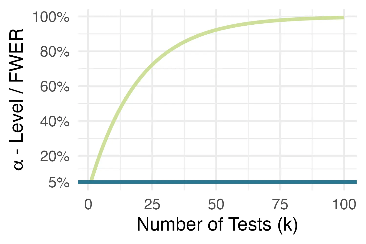
Thus, to avoid an inflation of false-positive findings, and to maintain the nominal significance level despite multiple testing, an \(\alpha\)-error correction is necessary. Let us illustrate this using our example trial data.
Imagine we hypothesized that, besides depressive symptom severity, our intervention also has effects on post-test behavioral activation and anxiety levels, as measured by the BADS-SF and HADS-A, respectively. Thus, we now want to confirm that our treatment is effective for three outcomes, and thus three tests have to be conducted. To test the effects, we run the same ANCOVA model already used in Section 4.1.3. For each outcome, we use its baseline measurement as the covariate in our model.
1with(implist, lm(cesd.1 ~ 1 + group + cesd.0)) %>%
    map_dbl(~anova(.)$`F value`[1]) %>%
    micombine.F(df1=1) -> F.cesd

2with(implist, lm(badssf.1 ~ 1 + group + badssf.0)) %>%
    map_dbl(~anova(.)$`F value`[1]) %>%
    micombine.F(df1=1) -> F.badssf

3with(implist, lm(hadsa.1 ~ 1 + group + hadsa.0)) %>%
    map_dbl(~anova(.)$`F value`[1]) %>%
    micombine.F(df1=1) -> F.hadsa

4(p <- c(F.cesd["p"], F.badssf["p"], F.hadsa["p"]))## p p p
## 4.062936e-16 1.521724e-03 5.369427e-08 The resulting \(P\) values are presented in scientific notation. For example, in the first value, the e-16 part tells us that the number should be multiplied with 10-16. As we can see, all of the \(P\) values are well below our threshold of 0.05, which means that we would conclude that the intervention was effective.
Yet, of course, these tests have not been corrected for multiple testing yet, which means that our \(\alpha\) level is inflated. Two commonly used methods to adjust for this are the Bonferroni and Holm-Bonferroni (Holm 1979) correction. The “classical” Bonferroni correction is overly conservative; while correcting for the type I error, it increases the probability of a type II error (i.e., it inflates our risk of keeping the null hypothesis, even when there is a real effect). The Holm-Bonferroni corrects for exactly this problem and may therefore often be preferable in practice unless avoiding false positives is extremely important.
In R, both methods can be implemented using the p.adjust function. We only need to provide the vector of \(P\) values that should be adjusted for multiple testing, as well as the method we want to apply:
p.adjust(p, method = "bonferroni")## p p p
## 1.218881e-15 4.565173e-03 1.610828e-07 p.adjust(p, method = "holm")## p p p
## 1.218881e-15 1.521724e-03 1.073885e-07 We see that, for both methods, the corrected \(P\) values remain well below 0.05. Thus, we can conclude that our intervention had effects not only on depressive symptom severity but also on behavioral activation and symptoms of anxiety.
The merits of multiplicity adjustments remain a controversial topic in clinical trial evaluations and elsewhere (Rothman 1990; Althouse 2016; Gelman, Hill, and Yajima 2012; Gelman and Loken 2013). The idea of \(\alpha\) correction is closely linked to the frequentist branch of statistics; Bayesian statisticians think quite differently about this topic (Sjölander and Vansteelandt 2019; Gelman, Hill, and Yajima 2012).
Althouse (2016) summarizes a few of the logical inconsistencies of multiplicity adjustments that have been described in the literature. A core criticism is that the number of tests we should adjust for is very much open to interpretation. Should it be for all tests conducted within a specific paper? This would mean that we can avoid adjusting our \(P\) value if we simply publish a separate paper for each hypothesis that we have. Such an approach would also “punish” larger, resource-intensive trials, since they typically include more outcomes than exploratory trials. What if other researchers also work on our trial data–should we adjust for their tests as well?
At the most extreme, we would have to adjust for all tests we expect to conduct during our scientific career. This would evidently be absurd, apart from being practically impossible.
Despite the logical inconsistencies we described in the box above, multiple testing can indeed jeopardize our inferences in certain contexts, so we have to draw the line somewhere. Below, we summarize a few practical recommendations on how to deal with multiple testing in practice (Li et al. 2017):
Multiple outcomes: A correction is only necessary if all outcome tests are considered confirmatory. If there is only one primary and several secondary endpoints, no correction is necessary. However, the results of secondary endpoints are only exploratory, not confirmatory evidence! They cannot “prove” that the intervention is effective for these outcomes, and further studies are needed to confirm that it is.
Multiple assessments: If only one assessment point is pre-specified as confirmatory-primary, no correction is necessary; likewise for tests where modeling is performed across multiple measurement points (e.g. using mixed models). In the next section, we will describe in greater detail how to deal with longitudinal data.
Multiple intervention groups: A correction is necessary when the intervention groups are “related” (e.g., the same medication at different doses; or the same self-guided intervention with and without human support). Adjustments may be of less importance when the interventions are clearly distinct (e.g. antidepressants versus cognitive-behavioral treatment, where both are provided as monotherapies).
Nowadays, in most mental health research RCTs, patients are followed up multiple times to assess how effects develop over time. For psycho-behavioral interventions, a frequently used method is to include a post-test assessment as well as (one or multiple) long-term follow-ups. Post-test assessments are usually conducted around the time the intervention is expected to be completed, while long-term follow-ups allow to check if the effects stabilize over time. In pharmacological research, it is also commonplace to have multiple visits to determine how patients respond over time.
As we discussed, clinical trials usually have only one primary endpoint, which is strictly defined as one specific comparison, measured by a specific instrument, at or within a specific time. Thus, if we have multiple measurements within the trial period of interest, these must be incorporated into a single analysis model to avoid multiple testing. There are several recommended approaches to analyze longitudinal data in RCTs, first and foremost linear mixed-effects models and generalized estimating equations (GEE, J. W. R. Twisk 2021, chap. 3.4). Here, we will showcase a longitudinal analysis using a special type of mixed-effects model known as mixed-model repeated measures (MMRM, Mallinckrodt et al. 2008).
Like conventional mixed models, MMRMs allow us to explicitly model that multiple assessments are available for each patient, and that these values are therefore correlated. In a “vanilla” mixed-effects model, this nested data structure (assessment points-in-patients) is often modeled by including a random intercept for each patient. These random intercepts are assumed to follow a normal distribution with mean zero and variance \(\tau^2\). Let us briefly flesh this out in a model formula:
This equation tells us that the outcome \(Y_{it}\) of person \(i\) at assessment point \(t\) is predicted by two types of regression terms: the fixed effects captured by the regression coefficients \(\beta\), as well as the random participant effect captured by the \(u_i\) term. The latter is a participant-specific value that shifts the intercept \(\beta_0\) up or down for that specific person, and the formula above is therefore known as a random intercept model.
We can also see that the fixed terms are equivalent to the ones we used in the linear ANCOVA model in Section 4.1.1: we have one coefficient for the effect of our treatment \(T\), while \(\beta_2\) captures the effect of the baseline covariate \(X\). Naturally, this model could also include more than one baseline covariate.
MMRMs try to capture the dependencies in longitudinal data in a slightly different way. They do not include special random effects in the model, but instead, specify that the residual errors \(\epsilon_{it}\) are correlated in a particular way. Equation 5.2 then simplifies to:
The special part of this equation is that we now allow for patient-specific variance-covariance matrices \(\boldsymbol{\Sigma_i}\), which are assembled in a block-diagonal matrix \(\boldsymbol{\Omega}\). Unstructured variance-covariance matrices of this form can be used within MMRMs to model the dependencies in our data, which removes the need to include random effects in the formula above.
This was a brief and somewhat technical introduction. The main takeaway is this: in RCT evaluations, we are typically only interested in fixed effects (e.g. the overall effect of our treatment). MMRMs allow us to estimate exactly that in longitudinal data, without the need to specifically define random effects, and while accounting for the dependencies in our data.
To illustrate MMRMs in practice, we will use the mmrm function, which is included in the eponymous package (Sabanés Bové et al. 2023). We will use this function to perform a longitudinal analysis of treatment effects on depressive symptoms, which were measured at a 7-week post-test (cesd.1) and 12-week follow-up (cesd.2).
To do this, we first have to transform our imputed data sets included in implist into the long format. We have already done this before in Section 3.2.3, where we prepared our data for the reference-based imputation, and similar code can also be applied here. We save the result as implist.long:
implist %>%
  map(function(x){
    x %>%
      mutate(id = 1:nrow(x)) %>%
      pivot_longer(ends_with(c(".1", ".2")),
                   values_to = "value",
                   names_to = c("outcome", "time"),
                   names_pattern = "(.*).(.)") %>%
        mutate(time = recode(time, `1` = 7, `2` = 12))
  }) -> implist.long
Let us have a look at the resulting data format:
# Extract a slice of the first imputed data set
implist.long[[1]][1:10, c("id", "outcome", "time", "value",
"cesd.0", "badssf.0", "hadsa.0")]## id outcome time value cesd.0 badssf.0 hadsa.0
## 1 1 badssf 7 20 24 24 7
## 2 1 hadsa 7 5 24 24 7
## 3 1 cesd 7 33 24 24 7
## 4 1 badssf 12 18 24 24 7
## 5 1 hadsa 12 10 24 24 7
## 6 1 cesd 12 30 24 24 7
## 7 2 badssf 7 24 38 33 11
## 8 2 hadsa 7 11 38 33 11
## 9 2 cesd 7 38 38 33 11
## 10 2 badssf 12 28 38 33 11We see that there are now several rows for each participant as indicated by the id variable. For each patient, we have follow-up data from two measurement points (time=7 and time=12), with three outcomes (badssf, hadsa, and cesd) each. Importantly, the baseline covariates are stored as separate columns and have constant values within patients.
For this analysis, we are only interested in the cesd outcome. Thus, we have to extract this outcome from all imputed data sets. We also convert the id, group, and time variables to factors, since this is a requirement of the mmrm function.
implist.long %>%
  map(~ filter(., outcome == "cesd") %>%
        mutate(id = as.factor(id),
               group = as.factor(group),
               time = recode(time, `7` = "7 wks", `12` = "12 wks") %>%
                 as.factor())
      ) -> implist.long
Now, let us fit our first MMRM model. For now, we focus only on the first imputed data set. As fixed terms in our formula, we include group and the baseline CES-D values, as we did in previous models. Then, we use the us function1 in the formula to specify the variance-covariance structure. Here, we use a model that also allows the variance-covariance matrices to vary between trial arms, which leads to us(time|group/id).
Additionally, we set the method argument to "Kenward-Roger", which means that the method by Kenward and Roger (1997) is used to construct confidence intervals and perform statistical tests. This approach is especially recommended for smaller data sets. We save the results as m.mmrm, and then plug this object into the summary function:
library(mmrm)
m.mmrm <- mmrm(value ~ group + scale(cesd.0) + us(time|group/id),
               method = "Kenward-Roger", data = implist.long[[1]])
summary(m.mmrm)## [...]
## Coefficients:
## Estimate Std. Error df t value Pr(>|t|)
## (Intercept) 22.9220 0.3965 271.8000 57.814 <2e-16 ***
## group1 -6.0220 0.5435 540.8000 11.080 <2e-16 ***
## scale(cesd.0) -0.2975 0.2727 542.7000 1.091 0.276
## ---
## Signif. codes: 0 ‘***’ 0.001 ‘**’ 0.01 ‘*’ 0.05 ‘.’ 0.1 ‘ ’ 1
##
## Covariance estimate:
## Group: 0
## 12 wks 7 wks
## 12 wks 105.2159 -1.7908
## 7 wks -1.7908 74.8074
## Group: 1
## 12 wks 7 wks
## 12 wks 85.8970 -2.9045
## 7 wks -2.9045 71.8065This provides us with an estimate of the intervention effect across the 12-week study period, \(\hat\beta_{\textsf{group}}=\) –6.02. Below, we are also presented with the (co)variance estimates for the two groups across both measurement points.
To fit this model in all imputed data sets, we can use the map function. Then, as before, we pool the parameter estimates using the testEstimates function in the mitml package:
implist.long %>%
  map(~ mmrm(value ~ group + scale(cesd.0) + us(time|group/id),
             method = "Kenward-Roger", data = .)) %>%
testEstimates()## [...]
## Estimate Std.Error t.value df P(>|t|) RIV FMI
## (Intercept) 23.022 0.473 48.698 483.087 0.000 0.467 0.321
## group1 -6.082 0.616 -9.865 815.571 0.000 0.325 0.247
## scale(cesd.0) -0.224 0.307 -0.730 838.243 0.466 0.319 0.244
## [...]This leaves us with a very similar estimate of the treatment effect, \(\hat\beta_{\textsf{group}}=\) –6.082, which is significant (\(p<\) 0.001). To derive a standardized effect size (i.e., Cohen’s \(d\)), we have to divide this estimate by the pooled standard deviation (see Section 4.1.4). A simple way to obtain this value would be to take the average of \(s_{\textsf{pooled}}\) in both measurement points. We omit this step here.
Next, we can also fit a slightly more sophisticated model in which the group term interacts with time. We can do this by joining group and time together with an asterisk (*):
implist.long %>%
  map(~ mmrm(value ~ group*time + scale(cesd.0) + us(time|group/id),
             method = "Kenward-Roger", data = .)) %>%
testEstimates()## [...]
## Estimate Std.Error t.value df P(>|t|) RIV FMI
## (Intercept) 22.555 0.757 29.799 531.492 0.000 0.436 0.306
## group1 -4.769 0.977 -4.881 833.057 0.000 0.320 0.244
## time7 wks 0.785 0.980 0.801 659.669 0.424 0.375 0.275
## scale(cesd.0) -0.224 0.307 -0.730 838.244 0.466 0.319 0.244
## group1:time7 wks -2.355 1.341 -1.757 794.252 0.079 0.330 0.250
## [...]The output is a little more difficult to decipher now. Since time is a factor variable, it is automatically dummy-coded by the function; and since "12 wks" comes alphabetically before "7 wks", it is used as the reference category in this model. This means that group1 now represents the treatment effect after 12 weeks (i.e., when time=0). We see that this value is slightly lower than the combined estimate (\(\hat\beta=\) –4.769) but still significant. This lets us conclude that the effects of treatment taper off slightly with time, but are still largely maintained after twelve weeks.
To obtain the effect estimate after 7 weeks, we need to look at the "group1:time7 wks" term. This tells us by how much we must adjust the “original” estimate captured by group1 to get the effect after 7 weeks. We can do this by adding the two point estimates together, which gives –4.769 – 2.355 = –7.124. This is the average treatment effect at post-test based on our model.
Unfortunately, since the 7-week effect is only defined in reference to the one after 12 weeks, its \(P\) value can not be interpreted as a test of the treatment effect itself. We see that the effect of "group1:time7 wks" is not significant (\(p=\) 0.079), but this only means that the treatment effects after 7 and 12 weeks do not differ significantly from each other.
To test the average effect after 7 weeks, we can use a little trick. In all of our imputed data sets, we recode the factor levels so that "7 wks" now comes before "12 wks", and is therefore used as the new reference category. This can be achieved using the levels argument in the factor function, where we have to provide the factor levels in the exact order in which we want them to appear. We save this model as m.mmrm.7wk. This leads to the following code:
implist.long %>%
  map(~ mutate(., time =
                 factor(time, levels = c("7 wks", "12 wks")))) %>%
  map(~ mmrm(value ~ group*time + scale(cesd.0) + us(time|group/id),
             method = "Kenward-Roger", data = .)) %>%
  testEstimates() -> m.mmrm.7wk

m.mmrm.7wk## [...]
## Estimate Std.Error t.value df P(>|t|) RIV FMI
## (Intercept) 23.340 0.613 38.050 586.915 0.000 0.406 0.291
## group1 -7.124 0.851 -8.376 770.393 0.000 0.337 0.254
## time12 wks -0.785 0.980 -0.801 659.670 0.424 0.375 0.275
## scale(cesd.0) -0.224 0.307 -0.730 838.242 0.466 0.319 0.244
## group1:time12 wks 2.355 1.341 1.757 794.253 0.079 0.330 0.250
## [...]As we can see, the 7-week assessment now serves as the reference group, to which the 12-week assessment is compared. The group1 term now directly shows us the 7-week effect (–7.124), where the point estimate is identical to the one we derived in the previous model. However, now we are also presented with a statistical test for this term, which tells us that the effect is also significant (\(p<\) 0.001). Like in Section 4.1.4, we can also use the confint function here to obtain valid confidence intervals around this estimate:
confint(m.mmrm.7wk)## 2.5 % 97.5 %
## [...]
## group1 -8.7934372 -5.4542877
## [...]To calculate confidence intervals for the 12-week effect, we would have to plug the previous model into the confint function instead.
In our longitudinal analysis above, MMRMs were fitted in the multiply imputed data, and we then calculated the pooled parameter estimates. Some researchers would probably disagree with this approach and argue that mixed models alone are already sufficient to deal with missing values under the MAR assumption (see Section 3.1.2), meaning that multiple imputation is not needed here.
It has indeed been found that linear mixed models can provide valid estimates under MAR even without multiple imputations (J. Twisk et al. 2013), and this approach is now commonly seen in practice. Unfortunately, this is often used as a blanket statement to argue why multiple imputation was not considered. In practice, things are often a little more difficult.
In Section 3.2.1, we learned that multiple imputation models should include auxiliary variables to increase the plausibility of the MAR assumption. If we do not use multiple imputation, this task is left to the mixed model itself, and how it is specified. In the MMRM model we fitted above, only baseline symptoms were used as a covariate. We presume that most longitudinal models in practice will not include many more variables than this either. Yet, to satisfy the MAR assumption, we need covariates that predict dropout, and it is questionable if this can be explained by the 1 or 2 covariates we typically include in a mixed model.
This problem can be solved by building a multiple imputation model with plausible predictors of missingness first and then fitting a mixed model in the multiply imputed data that actually addresses our research question. Another advantage is that we can also fit the same type of model to data sets that have been imputed under varying assumptions. For example, we could have also conducted an additional analysis within the “jump-to-reference”-imputed data (see Section 3.2.3) to assess longitudinal effects under an MNAR assumption.
We refer the reader to Magnusson (2019) for a more detailed explanation of the argument we presented here.
In the final section of our tutorial, we want to provide a little guidance on how to report the results of an RCT evaluation in a scientific paper. As we mentioned before (see Chapter 2, the CONSORT guidelines and checklist should be seen as minimal standards that every RCT report should follow. Besides the CONSORT flow chart we created in Chapter 2, our article should also include a table with descriptives for all measured variables. In the following, we provide a worked example of how to create such a table based on our multiply imputed data.
For the code below to work, we have to let R “learn” a function that we have written specifically for this purpose. To do this, you have to copy the code available here in its entirety, paste it into your R Studio console, and then hit Enter. Please note that the function requires the skimr, dplyr, and purrr packages to be installed on our computer.
In the following, we want to create a descriptive table for the intervention group, control group, and for our entire sample. As a first step, we have to define the number of imputation sets m that we created, as well as a vector with the names of all categorical variables (e.g. sex, employment, …) that we save under the name catvars.
m <- length(implist)
catvars <- c("sex", "prevpsychoth", "prevtraining",
             "child", "employ", "rel", "degree", "group")
Next, we make sure that all these categorical variables are converted to factor vectors:
implist %>%
  map(~mutate_at(., catvars, as.factor)) -> implist
Then, we can use the skimReport function that we just saved in our environment to create the descriptive tables for the complete sample (num.desc.full), intervention group (num.desc.ig), and control group (num.desc.cg). The code below is somewhat involved but should be easy to reuse for other multiply imputed data, as long as it is saved as an mitml.list with the name implist.
implist %>%
  map(~skimReport(.)) %>%
  {.[[1]]$numerics[,1] ->> var.names;.} %>%
  map(~.$numerics[,2:4]) %>%
  Reduce(`+`, .)/m -> num.desc.full

implist %>%
  map(~filter(., group == 1)) %>%
  map(~skimReport(.)) %>%
  map(~.$numerics[,2:4]) %>%
  Reduce(`+`, .)/m -> num.desc.ig

implist %>%
  map(~filter(., group == 0)) %>%
  map(~skimReport(.)) %>%
  map(~.$numerics[,2:4]) %>%
  Reduce(`+`, .)/m -> num.desc.cg
Lastly, we bind the three objects together to create the complete table.
tab.desc <- cbind(var.names, num.desc.full, num.desc.ig, num.desc.cg)
tab.desc## var.names mean sd n mean sd n mean sd n
## [...]
## 5 cesd.2 20.170 10.217 546 17.786 9.397 273 22.555 10.454 273
## 6 cesd.1 19.777 9.292 546 16.216 8.642 273 23.339 8.528 273
## 7 age 28.245 11.332 546 28.179 11.647 273 28.311 11.029 273
## 8 cesd.0 26.609 7.129 546 26.604 6.990 273 26.615 7.278 273
## [...]As we can see, this gives as the mean, standard deviation and sample size for all continuous outcomes at all measurement points. The left part of the table represents the full sample, the center the intervention group, while the right part contains descriptives for the control group.
If the openxlsx package is loaded, we can also save this table as an MS Excel file using the write.xlsx function:
library(openxlsx)
write.xlsx(tab.desc, file="imputed_descriptives.xlsx")
Another frequently asked question is how to report the results of the main effectiveness analysis. In most trials, multiple ANCOVAs are run, either because there were several primary endpoints, or because exploratory outcomes were also analyzed. In this case, it makes sense to assemble the results in a table.
Say that we want to report the results of the analysis in Section 5.1, in which we treated depressive symptom severity (measured by the CES-D), behavioral activation (measured by the BADS-SF) and HADS-A anxiety as co-primary endpoints. One way to do this is to create a table like the one below:

This provides us with the core outcomes of our linear regression model and ANCOVA: the estimated treatment coefficient \(\hat\beta_{\textsf{treat}}\) along with its standard error, as well as the fraction of missing information (FMI) and relative increase in variance (RIV) value. The next section displays the results of the \(F\)-test, and the last part gives the calculated effect size and confidence interval.
Although “open science” practices have become increasingly prevalent in many fields, the sharing of code and data in publications of mental health RCTs remains quite rare. The International Committee of Medical Journal Editors (ICMJE) released a statement that effective 2018, mandates a data-sharing statement for all clinical trials (Taichman et al. 2017). However, this does not mandate data sharing itself, and a large gap between the declared and actual availability of data has been found in the literature (Naudet et al. 2018; Danchev et al. 2021).
This is unfortunate; open research materials are usually an excellent way to allow others to examine how we arrived at our results, and facilitate their reproducibility. One way to make research materials openly available is to create an online repository on the OSF (Open Science Framework; osf.io). This allows to upload the R code we used for the analysis, as well as the de-identified trial data itself, and to state under which conditions other researchers can use it. Data sharing is especially helpful for meta-analytic researchers, who often require individual participant data (IPD) of several trials to examine treatment effects across different contexts.
If you decide to make your trial data publicly available, you may also consult the FAIR principles, which state that digital data sets should be Findable, Accessible, Interoperable, and Reusable.
\(\blacksquare\)
“us” stands for unstructured (variance-covariance matrix).↩︎