Having completed our descriptive analysis, we have now had the chance to familiarize ourselves with the structure of our data, as well as some of the patterns we find in it. Most importantly, we have found out that roughly 30% of all data at the post and follow-up assessment are missing. Missingness of this magnitude is not uncommon in “real-world” evaluations of psychological interventions, but this does not imply that we should take it lightly. In the primer article, we described that missing data poses a real risk to the validity of RCTs. We do not know for sure which mechanism created the missing data; but if the data are not missing completely at random and we do not account for that, it is very much possible that our estimates will be biased.
In the next section, we will therefore take some time to discuss how missing data mechanisms are typically classified in the literature, and what implications this has on our analysis. You might be wondering why we are making such a fuss about missing data. The reason is that some degree of missing data is almost unavoidable, even in relatively controlled designs such as RCTs; and that the way missing data is currently handled in (mental) health trials still leaves much room for improvement (see Table 1 in the primer paper for an overview). Unfortunately, R does not provide adequate missing handling “out-of-the-box” either. Let us illustrate that with a little example. Below, we fit a simple linear model using the lm function. Our dependent variable y is regressed on x, but x has a few missings:
# Define some example data; x has three missingsy <-1:10x <-c(1, NA, NA, NA, 3, 5, 8, 10, -1, 10)summary(lm(y ~ x))
Show result
## [...]## Estimate Std. Error t value Pr(>|t|) ## (Intercept) 4.9403 1.7738 2.785 0.0387 *## x 0.3172 0.2709 1.171 0.2945 ## ---## Signif. codes: 0 ‘***’ 0.001 ‘**’ 0.01 ‘*’ 0.05 ‘.’ 0.1 ‘ ’ 1#### Residual standard error: 2.904 on 5 degrees of freedom## (3 observations deleted due to missingness)
The most important information can be found in the last line, in which R tells us that the three observations were discarded before the model was fitted, a strategy that is also known as listwise deletion. This is a common ad hoc solution to deal with missing data in practice and is still often found in mental health research. However, it is not a recommended way to deal with loss-to-follow-up in randomized trials.
3.1 Missing Data Mechanisms
The way statisticians think about missing data has been shaped in large measure by the seminal work of Donald Rubin (Rubin 1976; van Buuren 2018, chap. 2.4.4). The core tenet of Rubin’s framework is that the presence and absence of observed data is the result of a probabilistic process. Our goal as analysts is to approximate this process using an adequate missing data model.
According to Rubin, these missing data models fall into three “prototypes”, which make different assumptions as to why some values were observed, while others “went missing”. We already mentioned these subtypes in the primer article, where we learned that data can either be missing completely at random (MCAR), missing at random (MAR) or missing not at random (MNAR). We will now take some time to discuss these types of missingness in greater detail, and what implications they have when analyzing RCT data.
Before doing so, let us introduce some common notation. We are aware that equations such as the ones we are about to discuss can seem frightening at first, but they are actually an excellent way to describe precisely the idea behind these different missingness mechanisms, so bear with us. First, let us list the “ingredients” we need to define each mechanism:
\(\mathbf{Y}\): The variables in our data set, which contain partially missing data: \(\mathbf{Y} = (\mathbf{Y}_{\textsf{obs}}, \mathbf{Y}_{\textsf{mis}})\).
\(\mathbf{Y}_{\textsf{obs}}\): All the values in \(\mathbf{Y}\) which were actually observed (i.e., are not NA).
\(\mathbf{Y}_{\textsf{mis}}\): The values in \(\mathbf{Y}\) which were not observed, but exist in theory.
\(\mathbf{R}\): A matrix of the same size as \(\mathbf{Y}\), but which only consists of 0’s (value missing) und 1’s (value observed). This is also known as the “response indicator”.
\(\psi\): Parameters of the missing data model (these parameters are typically not relevant to the scientific question itself).
Using these parameters, we can assemble a general formula that builds the basis of all missingness mechanisms:
As indicated by the \(P\) up front, this is a conditional probability, where the \(|\) part can be read as “given”. Taken together, the formula tells us that every missingness model should give us the probability of some value not being recorded (\(\mathbf{R}=0\)), given the observed data \(\mathbf{Y}_{\textsf{obs}}\), the missing values \(\mathbf{Y}_{\textsf{mis}}\), and some missing data model parameters \(\psi\) (which we can ignore for now).
This formula is quite abstract, but there is something important to draw from it. It tells us that all missingness mechanisms make some statements about how \(\mathbf{R}\), \(\mathbf{Y}_{\textsf{obs}}\) and \(\mathbf{Y}_{\textsf{mis}}\) relate to each other. As we will illustrate in the next sections, the main difference between the mechanisms is the degree to which they allow the formula above to be “simplified” by removing \(\mathbf{Y}_{\textsf{obs}}\), \(\mathbf{Y}_{\textsf{mis}}\), or both \(\mathbf{Y}_{\textsf{obs}}\)and\(\mathbf{Y}_{\textsf{mis}}\) from the equation.
3.1.1 Missing Completely At Random (MCAR)
If the data are missing completely at random (MCAR), we assume that the missingness of values (as encoded by \(\mathbf{R}\)) is completely independent of \(\mathbf{Y}\). As it says in the name, we believe that missings occurred in a fully random fashion; they are neither associated with any of the observed data \(\mathbf{Y}_{\textsf{obs}}\), nor with the unobserved values \(\mathbf{Y}_{\textsf{mis}}\). Equation 3.1 from before can therefore be simplified like this:
which tells us that the response indicator only depends on \(\psi\), which can be interpreted as the overall missingness probability (i.e., there generally tend to be many or rather few missings in the data). It is quite clear that this is a very strong assumption, which may not be very plausible in practice.
3.1.2 Missing at Random (MAR)
The missing at random (MAR) assumption presumes that the missingness of values denoted by \(\mathbf{R}\) does depend on some information in \(\mathbf{Y}\), but in a special way. We assume that \(\mathbf{R}\) only depends on the observed information \(\mathbf{Y}_{\textsf{obs}}\), so that \(\mathbf{Y}_{\textsf{mis}}\) drops out of the equation:
Put differently, the MAR assumption states that, by using all the information in the observed data, we can accurately describe why some values are missing. After controlling for these factors, the data are missing completely at random again. We also assume that the missing values \(\mathbf{Y}_{\textsf{mis}}\) themselves carry no special information beyond what is already captured by \(\mathbf{Y}_{\textsf{obs}}\), which is why they can be removed from the equation.
3.1.3 Missing Not at Random (MNAR)
The missing not at random (MNAR) assumption is the most general of the three “prototypes”. When the data are MNAR, we assume that the missingness indicator \(\mathbf{R}\) depends on both \(\mathbf{Y}_{\textsf{obs}}\)and\(\mathbf{Y}_{\textsf{mis}}\). If this is the case, there is no way to further simplify Equation 3.1:
The main implication of the MNAR assumption is that the missingness of our data as encoded by \(\mathbf{R}\) does, at least to some extent, depend on the values of the missing data \(\mathbf{Y}_{\textsf{mis}}\)themselves. As analysts, this brings us into somewhat of a conundrum: it means that, if our missing data model should accurately reflect the reality behind our data, we have to account for the information included in \(\mathbf{Y}_{\textsf{mis}}\); but this is impossible because the information in \(\mathbf{Y}_{\textsf{mis}}\) has never been recorded. The fact that these values are missing is the exact reason why we need a missing data model in the first place.
This may sound paradoxical, but there are many scenarios, including RCT evaluations, where the MNAR assumption is very much plausible. Let us assume, as we did in the primer article, that patients did not provide outcome data in the intervention group because they did not experience any benefits of the intervention. In this case, it is likely that our measurement of the outcome (say, depressive symptom severity) is missing precisely because of its value. Some patients still experience very high levels of depression, and that is why their depression score was not recorded. We can then say that the data in our trial are MNAR.
3.1.4 Implications
What implications do these different missing data mechanisms have on our analysis? If our data are really MCAR, the answer is straightforward: there will be no systematic bias in our estimates; we only lose statistical power (i.e., we have to live with broader confidence intervals) because some of the data is missing.
Things get more complicated if the data are MAR. Here we assume that values are missing at random conditionally on other variables, meaning that our estimates will be biased if we look at some variable in isolation. Imagine that \(Y\) is the primary outcome of our trial (like the CES-D score at post-test in our example data). If the data are MAR, summary statistics calculated from \(Y\) (e.g. the mean in the treatment and control group) will be biased. However, if we adjust for the information included in other observed variables, this bias can be avoided. One (of several) ways to achieve this is by constructing an imputation model that makes use of this information in our data, as we will do in Section 3.2.
From an analytic perspective, MNAR data arguably poses the greatest challenge. If the data are truly MNAR, our estimates are likely biased, and there is no information within our data to “rescue” our analysis. We can only hypothesize how and how strongly the underlying missing data model plausibly departs from the MAR assumptions, and implement statistical approaches that represent these “best guesses”. In an individual study, there is no way to prove that our chosen approach to handling MNAR data is adequate; just as it is also not possible to prove that our data are MNAR in the first place. We quote from Molenberghs et al. (2004), p. 447:
“MNAR models are […] typically highly dependent on untestable and often implicit assumptions regarding the distribution of the unobserved measurements given the observed measurements.”
Overall, this underlines the importance of sensitivity analyses: by considering the impact of various plausible missing data assumptions on our results, we can make more qualified statements on the robustness of our findings. Methods to handle MNAR data are an open research topic, and several approaches are available. We will cover some of them in Section 3.2.3.
One last distinction we want to introduce here is the one between ignorable and non-ignorable missing data. If data are MCAR or MAR, we can say that our missing data are ignorable, while MNAR means that we have non-ignorable missing data. Please note that this is a technical term that does not imply that we do not have to “care” about our missings if they are MCAR or MAR. In fact, ignorability means that we can infer from the joint distribution of the observed data to one of the missing data. When the data are non-ignorable (i.e., MNAR), this assumption is violated:
Thus, if we are dealing with non-ignorable missings, an estimation (imputation) based on the available values is not possible without further ado; assumptions must be made that “go beyond the data”.
Which Missing Data Assumption Should I Make?
As mentioned, strictly speaking, there is no way to confirm if the missings in our trial data are ignorable or non-ignorable. Sometimes, differential dropout1 is taken as a sign of non-ignorable missing data, but that is not necessarily true: differential dropout can lead to biased results but does not have to; conversely, biased results are also possible even when dropout has been equal between groups (Bell et al. 2013). As we mentioned, sensitivity analyses that account for different plausible missing data mechanisms should be seen as a standard part of every RCT evaluation. This makes the question of which mechanism fits the present best less problematic than one may initially fear, as long as several plausible options are covered.
Nevertheless, when designing the statistical analysis plan of a trial, we have to define a priori what the “primary” our “main” effectiveness analysis of our trial will entail. This means that we have to choose some mechanism as a plausible starting point, even though we will accompany it with sensitivity analyses later. There are no iron-clad rules, but it has been frequently mentioned that an analysis assuming MAR may often be a good first start. Let us quote a few authoritative sources here:
“[W]e recommend that in trials […], all data should be used in an analysis that makes a plausible assumption about missing data. Usually, this will be a MAR assumption.” (Bell et al. 2014)
“The assumption of ignorability is often sensible in practice, and generally provides a natural starting point.” (van Buuren 2018, chap. 2.2.6)
“When […] a complete records analysis is insufficient, the framework suggests an analysis assuming MAR. This is because […] MAR is the most general assumption about the missing data distribution we can make without recourse to bringing in external information.” (Carpenter and Smuk 2021)
If we assume that the data are MAR, we should also choose a compatible missing data handling method. One option for this is multiple imputation, which we will cover in the next section.
A Few Remarks On Little’s MCAR Test
It is still quite common to see RCT evaluations in mental health research report the results of Little’s (1988)\(\chi^2\) test, often with the intention to “confirm” that the data are MCAR. This approach is flawed. Our null hypothesis in Little’s test is that the missings in our data appeared randomly, i.e., that the data are MCAR. Our ability to reject this null hypothesis depends on the statistical power of the test, which in turn depends on our sample size; this problem is exacerbated if the data are in fact MNAR (Thoemmes and Enders 2007); if we cannot reject the null hypothesis, this does not confirm that the data are in fact MCAR.
Even if the null hypothesis is rejected, this means that the data can either be MAR or MNAR. The difference between MAR and MNAR is much more important in practice because conventional missing data handling methods (e.g., most multiple imputation approaches) provide valid results under MAR, but not MNAR. Furthermore, as we learned above, MCAR is not a very plausible missing data assumption in RCTs to begin with, with the MAR assumption typically providing a better starting point.
Taken together, this should underline that the practical utility of Little’s MCAR test is very limited, and it is probably best to avoid using it in RCT evaluations altogether. A more comprehensive treatment of the problems with Little’s test is provided in (C. K. Enders 2010, 21).
3.2 Multiple Imputation
Multiple Imputation (MI, Rubin 1996, 2004) is one of the most flexible and commonly used methods for dealing with missing values. The goal of MI is to estimate (“impute”) plausible values for missing data, based on the distribution of the observed values.
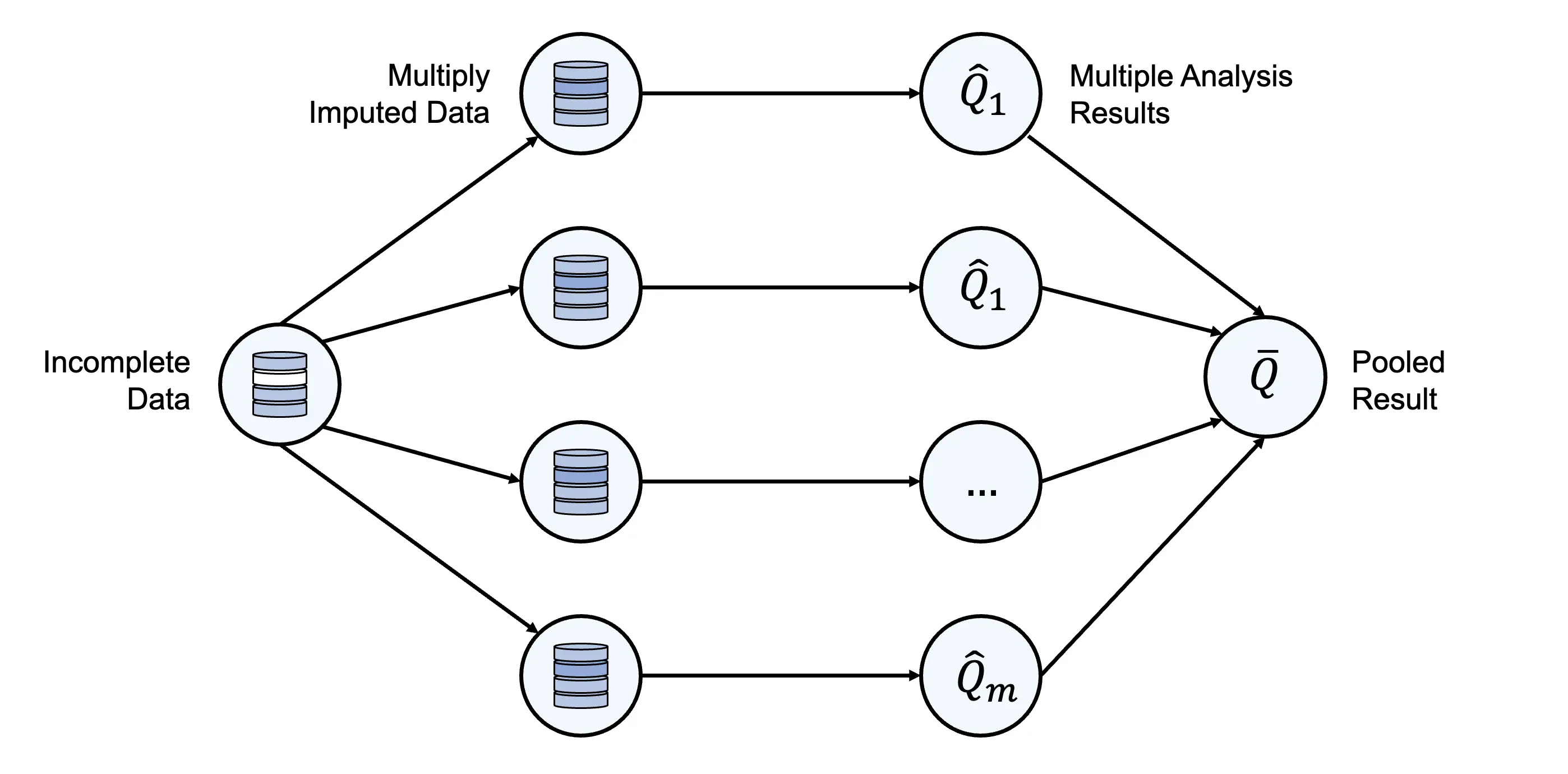
Importantly, as part of MI, we generate multiple imputations for each missing value to reflect the uncertainty of our estimation. The complete data sets generated in this way are then analyzed simultaneously (we could, for example, calculate a sample mean in all imputed data sets). In the end, all results are then pooled into one estimate.
MI can be used under the assumption of MCAR and MAR (and under certain conditions also MNAR). When applied correctly, MI results in an unbiased estimation of population parameters (regression weights, population means, correlations, etc.) and their variance (“asymptotically unbiased”) despite the presence of missing values (I. R. White, Royston, and Wood 2011a).
In terms of implementation, two broad “flavors” of MI can be distinguished:
Joint Modeling (JM): A multivariate distribution (“joint model”) for the missing data is specified, and imputations are sampled using Markov Chain Monte Carlo (MCMC, Schafer 1997).
Fully Conditional Specification (FCS): Incomplete variables are imputed in a sequential and iterative process, one variable at a time. Unlike JM, it is not necessary to find a multivariate distribution of the missing data for FCS. In this regard, FCS is “atheoretic”.
In this tutorial, we will focus on how to implement MI using fully conditional specification (FCS). We do this because FCS is a slightly more flexible method that translates well to new analytic tasks; and because it might slightly more convenient to apply for novice analysts. Joint modeling has other strengths, for example when dealing with clustering or other more complex data structures. Since JM is also more “theory-driven” than FCS, it can also have advantages in achieving what is known as “compatibility” or “congeniality” of the imputation model, a topic that we will cover in Section 3.2.3. An excellent way to implement JM in R is via the jomo package (Quartagno and Carpenter 2022a). A practical introduction to this package can be found in (Quartagno, Grund, and Carpenter 2019).
3.2.1 Multivariate Imputation By Chained Equations
The MICE (Multivariate Imputation by Chained Equations) algorithm is one of the most commonly used and best-studied FCS approaches. As it says in the name, MICE is based on the idea of chained equations, which is what we discuss now.
Imagine that we have a data set \(\mathbf{Y}\) that consists of \(p\) variables. We can write: \(\mathbf{Y} = Y_1, Y_2, ..., Y_p\). The values of the \(p\) variables are partly observed, and partly missing. When building our imputation model, we assume that these variables are created by \(\boldsymbol{\theta}\), an unknown vector of population parameters. This multivariate distribution of \(\boldsymbol{\theta}\) is what we want to approximate in order to generate accurate imputations.
The MICE algorithm achieves this implicitly, by sampling over each incomplete variable \(Y\) from its conditional distribution, in the following form (van Buuren and Groothuis-Oudshoorn 2011a):
Here, the subscript \(\setminus p\) indicates that all information in our data \(\mathbf{Y}\) is used to sample data for the missing values in some variable \(Y\), except the imputed values of \(Y\) itself. This is a special feature of the MICE algorithm.
MICE is implemented through a method called Gibbs sampling. Based on some starting values, \(\theta\) is estimated for each variable \(j\), which is then directly used to generate imputed values \(Y^{*}_{j}\). These values then form the basis for further sampling. This leads to the following set of “chained” equations for each iteration \(t\):
Typically, this process converges after a certain number of iterations and reaches stationarity (i.e., it “stabilizes” around a particular set of values). Since in MICE, the previous imputation \(Y^{t-1}_j\) is not directly used in the imputation of \(Y^{t}_j\), this is achieved relatively quickly (often after 5-10 iterations). This iterative process is performed multiple times in parallel to generate the \(m\) imputation sets.
Equation 3.7 above is complex, and it is not necessary to understand every detail of it. What matters is that the formula reveals something special about the MICE algorithm and FCS in general. While we assume that there is some complex multivariate distribution \(\boldsymbol{\theta}\) that generated our data, MICE does not try to approximate this distribution directly through some joint model (like JM), but instead defines a separate model for each variable individually. This makes the MICE algorithm somewhat “atheoretic”, but dramatically improves the flexibility of the approach, and makes it applicable to data with all kinds of variable types (continuous, binary, categorical). It has also been shown that MICE/FCS generally performs well across various contexts and data structures (Grund, Lüdtke, and Robitzsch 2018; van Buuren et al. 2006; van Buuren 2007; Craig K. Enders, Hayes, and Du 2018; de Silva et al. 2017), despite its atheoretic nature.
Our main task when using MICE in practice is thus to define an apt set of predictors for each imputed variable individually, as well as the method by which imputations should be generated. Table 3.1 provides an overview of commonly used imputation methods, as well as their implementation within the mice package (van Buuren and Groothuis-Oudshoorn 2011b) which we will also use in this tutorial.
Table 3.1: Commonly used imputation techniques for MICE, by data type
Model/Method
Implementationa
Data Type
Predictive Mean Matching
pmm
various
Bayesian Linear Regression
norm
continuous
Unconditional Mean Imputation
mean
continuous
Bayesian Logistic Regression
logreg
binary
Bayesian Polytomous Regression
polyreg
factorial
aName of the implementation within the mice package.
One of these methods, predictive mean matching(PMM, Morris, White, and Royston 2014), deserves a little further attention. PMM is a so-called “hot deck” method, which means that it imputes missings based on the real values recorded for other, but statistically similar individuals in our data. In essence, PMM involves a two-stepped procedure: first, we try to predict the values of a variable with missings using other recorded information in our data set; this allows us to create a predicted value for both the individuals that were actually observed, \(\hat{y}^{\textsf{(obs)}}_i\), and the predicted values of those whose true values were not observed, \(\hat{y}^{\textsf{(mis)}}_j\). Note that we use a hat symbol (^) to indicate that we are using predicted values of \(y\).
In the next step, we gauge these predicted values to identify “donors” for each person with missing values. Donors are individuals without missings whose predicted values \(\hat{y}_i\) are similar to the one of an individual with missing data. Put differently, our goal is to find participants with recorded data on \(y\) whose predicted values deviate as minimally as possible from the predicted values of the person for which \(y\) has to be imputed:
In most cases, \(d\)=3-10 donor candidates are identified this way, and one is then selected randomly to “donate” its recorded value to the person for whom no value was recorded. In the mice package, 5 donor candidates are used by default.
PMM is a broadly applicable and typically robust technique for imputations. One of its perks is that it can be used for various data types, including continuous, binary, and categorical variables. Furthermore, since all values come from observed donors, imputing “impossible” values (e.g., an age of -2) is ruled out a priori.
Multiple Imputation using MICE: A Few General Tips
Number of imputation sets. Typically, generating \(m\)=20 imputations is already sufficient when the amount of missing data is moderate. However, more imputations may be necessary if the goal is to precisely estimate parameters that are often difficult to estimate (e.g., standard errors or variance components); or when there is a large number of missings (van Buuren 2018, chap. 2.8). In most practical contexts, the time needed for the imputation will be manageable even when the number of imputations is set to a higher value, so using \(m\approx\) 50-100 imputations might generally be a good approach in practice.
Number of iterations. As mentioned above, a key feature of the MICE algorithm is that it converges quite fast, so that 20-30 iterations are often sufficient. A higher number can be chosen when it is unclear if the algorithm has converged. Section 3.2.2 covers how to diagnose convergence issues when using MICE, although some of these problems cannot be solved by simply increasing the number of iterations.
Number of variables. Another key question when building an imputation model is the number of auxiliary variables to be used for imputing missing values. First and foremost, variables should be used as predictors in our imputation model if they are plausibly related to the imputed variable(s) and/or their missingness. Including a wide range of meaningful auxiliary variables makes the MAR assumption more plausible, but also increases the complexity of our imputation model, which can lead to estimation problems. The goal is therefore to find a middle ground when the imputation model fails; i.e., to reduce its complexity without reducing the overall plausibility of the model. To quote I. R. White, Royston, and Wood (2011b):
“In general, one should try to simplify the imputation structure without damaging it; for example, omit variables that seem on exploratory investigation unlikely to be required in ‘reasonable’ analysis models, but avoid omitting variables that are in the analysis model or variables that clearly contribute towards satisfying the MAR assumption.”
3.2.2 MICE in Practice
After all this technical input, it is time to implement MICE in practice. To build our imputation model, the mice and miceadds(Robitzsch and Grund 2022) packages need to be installed and loaded from the library. The mice package is the main workhorse we use to set up and run our model, while the miceadds package provides additional helper functions.
library(mice)library(miceadds)
First, let us explore the missingness pattern in our data frame object data. We do this by plugging it into the md.pattern function, which creates the following output:
md.pattern(data)
This plot may be difficult to decipher at first, so let us go through it step by step. The rows in the plot above show the distinct missingness patterns, with the numbers to the left indicating how frequently each of them appears in our data. Within each pattern (i.e., row), a blue tile symbolizes that a specific variable (indicated by the columns) has been observed, while a red tile shows that the variable is missing.
This graphic makes it clear that we have three missingness patterns in our data. The first, and most common case (\(n\)=381 individuals) is that all variables have been recorded. The second case (\(n\)=10 individuals) is that the badssf.2, hadsa.2 and cesd.2 variables are missing, with the rest being recorded. This pattern coincides with all the patients in our trial who could not be reached at the 3-month follow-up. The last pattern, which is represented by \(n\)=155 patients, are individuals whose measurements are missing at both post-test and follow-up, but with all the baseline measurements being recorded.
This shows that our data displays what is known as monotone missingness: over time, some patients drop out of the trial and cannot be reached anymore, including at later assessment points. This means that the missings gradually increase over time; although, in our case, the number of additional missings at the 3-month follow-up is small. Such a missingness pattern is not uncommon in longitudinal studies in general, and randomized controlled trials in particular.
The next thing we examine is the so-called influx and outflux pattern of our missings. Using the flux function, an influx and outflux coefficient can be calculated for each variable, which can be helpful to determine variables that are more or less relevant for our imputation model. For two variables with the same amount of missingness, a higher influx and/or outflux coefficient means that the variable is more connected with the rest of the data, and might therefore be more relevant for our imputation model.
Calculating the Influx & Outflux Coefficient
The influx coefficient\(I_j\) of some variable \(j\) indicates how well missing values in \(j\) are covered by observed values in other variables; i.e., how much information of other variables can potentially “flow into” \(j\).
Let \(R_{ij}\) be the response indicator (1 = observed; 0 = missing) for some person \(i\) on some variable \(j\), and let \(R_{ik}\) be the response indicator for the same person on some other variable \(k\). The influx coefficient can then be calculated as (van Buuren 2018, chap. 4.1.3):
The outflux coefficient\(O_j\) indicates how well observed values in \(j\) can be used to cover missing values in other variables. For each variable \(j\), we get the following formula:
Let us inspect the results we obtain for our data set data. Please note that we add [,1:3] to our function call because we only require the first three columns of the output:
Looking at the output values, we see that many variables in our data have an influx coefficient of 0, while their outflux is 1, which is the largest possible value. This is because these are baseline variables, which, in our case, have no missings. Naturally, this means that all information is flowing “out” of these variables, while there is no influx. This could make these variables potentially very valuable as predictors in our imputation model.
We see a different pattern for the variables assessed at post-test and follow-up. Here, the outflux is very low (\(O_j\) = 0.03 for post-test variables) or zero altogether (for follow-up measurements). On the other hand, there is some influx for these variables, which is slightly larger for the follow-up variables, because they are covered by both the baseline variables and a few post-test measurements.
These results reveal that, since our RCT data displays monotone missingness, the heuristic value of the influx and outflux coefficient is somewhat limited; there is nothing particularly surprising about the results we obtained here. However, when the missingness is not (completely) monotone, the flux indices can indeed be helpful to identify variables that may be more or less helpful to use as predictors in our imputation model.
Limitations of the Flux Coefficients
The flux coefficients only tell us how well missing values in some variables are connected to observed values in others; they do not assess if a particular variable is actually predictive of another. Therefore, we should not rely on them alone to determine which variables to include in our imputation model.
As a last preparation step, we will explore if some of our (completely recorded) baseline variables are associated with the missingness of values at post-test (see e.g. Carpenter and Smuk 2021). This can be helpful to identify variables that we should consider including as predictors in the imputation model. To do this, we first create a response indicator R within our data set, which identifies if our primary outcome, the CES-D score at post-test, has been recorded or not. Then, we split the data by treatment group so that we can examine both separately. We name the resulting two data frames data.cg and data.ig:
data$R <-!is.na(data$cesd.1)data.cg <- data %>%filter(group ==0)data.ig <- data %>%filter(group ==1)# R is not needed for other analyses, so# we remove it from the original datadata$R =NULL
Now, we can run a logistic regression model that predicts response at post-test using our recorded baseline variables. This can be implemented in R using the glm function, in which we have to specify binomial(link = "logit") so that a logistic regression model is run. In the first argument, we provide the formula, in which we regress R on the baseline variables in data. Regression models specified in R often take the generic form y ~ x + z, which means that y is predicted by x and z.
In the formula argument, we use the scale function to center and scale all the continuous variables, which makes it easier to interpret the results. We also plug categorical variables into the as.factor function so that they are encoded as factors. This leads to the following code for the intervention group data:
As indicated by the asterisks there are several baseline characteristics associated with higher or lower odds that a patient will not be observed at post-test. We see, for example, that higher badssf.0 and hadsa.0 values make it less likely that patients’ post-test score was recorded. The same is true for participants who have previous psychotherapy experience, and this effect is even highly significant (\(p<\) 0.001). Lastly, we also see that values are more likely to be missing if a patient is widowed (rel=3).
There are several takeaways from these results. First, they underline that our data are unlikely to be MCAR; there seem to be systematic factors in the intervention group that predict if a person is more or less likely to drop out from the study. Second, we were able to identify some variables indicative of missingness that we should make sure to include as auxiliary variables in the imputation model.
Lastly, please note that we have mostly focused on the statistical significance of the examined predictors here; naturally, statistical significance also heavily depends on the size of a data set and therefore should not be the only criterion based on which plausibly relevant predictors should be included.
For comparison, let us also examine the results we obtain from the control group:
While fewer predictors are significant here, the overall pattern is quite similar. The main exception is the “widowed”-level of the rel, the regression coefficient of which has a different sign now, and is not significant anymore.
Based on these results, we can define an “inlist”, a selection of baseline variables that should always be included in our imputation model. Here, we choose the badssf.0, hadsa.0, prevpsychoth and rel variable:
We are now set and ready to initialize our MICE model for the first time. For now, we only provide our data set data and specify maxit = 0 within the mice function. This means that a “null imputation” is conducted: the data is checked for potential problems, but no actual imputations are generated. We save the result as imp0.
imp0 <-mice(data, maxit =0)
Show result
## Warning message:## Number of logged events: 1
The output tells us that there was one logged event. We can use the $ operator to inspect it:
imp0$loggedEvents
Show result
## it im dep meth out## 1 0 0 constant id
The function tells us that there is one constant in our data that cannot be used within the imputation model – our patient id. Since this variable does not carry any meaningful information anyway, we remove it from our data and save the new data frame as imp.data.
1outlist <- imp0$loggedEvents$out2imp.data <- data %>%select(-all_of(outlist))
1
Include all variables with logged events (“id” in our case) in our “outlist”.
2
Then, remove those variables from the data frame.
Using this new data frame, we can now use the quickpred function in mice to create a predictor matrix. This predictor matrix is the core of our imputation model and indicates which variables will be used as predictors for which variable with missing data. As we learned, MICE as an FCS approach gives us a lot of flexibility in defining this matrix, so it is important to put some thought into this step.
The quickpred function takes several relevant arguments that should be specified. First, we have to provide a value of mincor, the minimal correlation between a predictor and the imputed variable that is required for that predictor to be used in our imputation model. We set this value to \(r\)=0.05, which means that a predictor has to be at least slightly associated with the variable we want to impute; if this is not the case, the variable will be removed from the predictor matrix. The minpuc argument in the quickpred function follows a similar logic. It lets us define the minimum proportion of usable cases within a predictor when imputing another variable with missings. Here, we set this value to \(p\)=0.05, which means that at least 5% usable cases are needed and that the variable will be removed as a predictor if this is not the case.
The idea behind both mincor and minpuc is to a priori remove predictors that do not carry a substantial amount of meaningful information in imputing a variable with missings. This is a way to simplify our imputation model so as to avoid computational problems further down the line.
The last argument in quickpred we want to specify is include. This argument can take a selection of variables that should always be used to predict missing values. Previously, based on our inspection of the missingness pattern in both trial groups, we already defined our inlist of potentially important predictors, and it makes sense to provide this selection of variables within the function. We save the results of our call to quickpred as pred.
pred <-quickpred(imp.data,mincor =0.05,minpuc =0.05,include = inlist)
Next, we can inspect the matrix. As we learned before, a great asset of multiple imputation (and FCS in particular) is that it allows to integrate the information captured by auxiliary variables, which can help to make the MAR assumption more plausible. Naturally, this means that, for each missing variable, a sufficient amount of potentially meaningful predictors is used in our imputation model. To check this, we can calculate the mean number of predictors for each variable with missings, using the following code:
# Mean number of predictorstable(rowSums(pred))[-1] %>% {as.numeric(names(.)) %*% . /sum(.)}
Show result
## [,1]## [1,] 13.33333
The output shows that approximately 13 predictors are used to impute each variable with missings in our data. This is not too bad, given that our data frame dat.imp only has 20 variables.
As a next step, we have to slightly adapt the matrix. When imputing data of clinical trials, it is sensible to generate imputations seperately for the intervention and control group, because this allows to also capture patterns that might differ between the two groups. Some baseline variables in our data (e.g. depressive symptom severity, age, etc.) could be effect modifiers, which means that their influence on the imputed outcome differs between the two groups.
Imputing separately for both groups can help to address this issue. However, to implement a group-wise imputation, we first have to make sure our group variable is not used as a predictor in the matrix. This is because once we start to impute for each group separately, the group variable does not carry any information anymore (since it is either all 0 or all 1).
The remove the group variable from our imputation model, we have to set its column in the imputation matrix to zero, which we can do like this:
# Set predictor "group" to zeropred[,"group"] =0
Once these preparations are completed, we can also visualize the imputation matrix. To do this we have to make sure that the plot.matrix package is installed and loaded from the library. Then we can use the plot function to generate a graph:
library(plot.matrix)plot(pred, main ="Imputation Matrix",col =c("grey", "blue"),xlab ="predicts",ylab ="is predicted",adj =0, las =2, cex.axis =0.5)
This predictor matrix is the core of our imputation model, and it makes sense to include it in our RCT analysis report (for example in the supplementary material). This is because the matrix tells us exactly which predictors are used to impute which variable with missing values. To better understand its structure, it helps to go through each row of the matrix step by step. As indicated by the \(y\)-axis label, the rows tell us the variable that should be imputed, while the columns indicate the predictors that will be used. However, variables only serve as predictors when their respective field is highlighted in blue.
This allows us to observe a few general patterns. First, we see that the quickpred function selected most baseline co-variates as predictors for the missing post-test and follow-up assessments. One exception are prevtraining and degree, which have been removed for some variables based on their correlation and proportion of usable cases. Second, we see that predictors are only defined for a few variables within our data. These are the outcome assessments that actually have missings, while the rest are complete baseline measurements that do not have to be imputed.
Lastly, the matrix also points us to a weakness of our imputation model. To estimate missing values in the outcome variables, most of the information we can rely on is based on the baseline characteristics of a person. Only some post-randomization measurements can be used as predictors, which is the result of us setting the minimal proportion of usable cases to 5%. This is not uncommon with RCTs, in which data is often missing monotonously. This should remind us that multiple imputation is not a panacea and that we will need a few sensitivity analyses to assess the robustness of our results. We will elaborate on this point in Section 3.2.3 and Section 4.1.3.
With our predictor matrix set up, we now have to determine the imputation method we should use. As shown in Table 3.1, several techniques are available for this, and we have to decide which one fits best with the type of data we aim to impute. A good first start is to let mice preselect a fitting imputation method for us, which can then be changed if necessary. To do this, we have to run a null imputation again, but this time we already provide our predictor matrix in the predictorMatrix argument. We can then extract the method object, which contains the imputation technique that mice selected for us.
We see that for all variables with missings, predictive mean matching ("pmm") has been chosen. Given that all variables with missings are continuous, this might indeed be a good default strategy.
Alas, we are not done here. Since we want to impute separately for each group, our imputation method has to be slightly adapted. First, we create an index named no.missings, which indicates if a variable has no missings. This is true for all variables for which the imputation method was set to "" by mice.
# Find variables without missingsno.missings = imp0$method ==""
Next, we have to replace the imputation method of all variables with missings from "pmm" to "bygroup", which tells the mice function to impute separately by trial group. We save the resulting object as imp.method.
# Set imputation method to "bygroup"imp0$method %>%replace(., . !="", "bygroup") -> imp.method
Now that we have an object that tells mice to impute by groups, we also need another object which specifies the actual imputation technique used within each group. To do this, we extract all elements from the original vector of imputation techniques in imp0 associated with variables with missings, and then convert them to a list element. We save the resulting object as imp.function.
# Define the actual imputation method for all "bygroup" variables imp0$method[!no.missings] %>%as.list() -> imp.function
Lastly, we have to produce a list element that encodes the grouping variable for each imputed variable in our data (in our case, this is group). We can achieve this using the code below; please note that the purrr} package (Henry and Wickham 2020), which is part of the tidyverse, has to be loaded first for this to work. We save the resulting list as imp.group.variable.
Preparing these different lists and vectors is quite tedious. Fortunately, we now have all the ingredients we need to run our penultimate call to mice in which the data are finally imputed.
There are a few things to mention here. First, we specify the predictorMatrix argument again and provide our predictor matrix pred. In the method argument, we plug in our imp.method object, which tells mice that imputations should be performed by group. The imputationFunction argument is used to specify the actual imputation technique that is used within the two groups. In the group argument, we provide our list specifying the grouping variable for each outcome with missings.
The m argument specifies the number of imputed data sets we want to generate. Here, we use m = 50. Since we want to conduct an actual imputation now, we set the maxit argument, specifying the number of MICE iterations, to 50. Lastly, we can also specify a seed within mice. This allows us to offset R’s random number generator, which is helpful if we want to keep our results reproducible at a later stage. Please also note that the miceadds package needs to be loaded for the code below to work.
Warning
When specifying the mice function, please always make sure that its results are saved to an object using the assignment operator. If results are not assigned to an object, the imputation will run regularly, but the imputed data sets will not be saved. In our example below, we save the results as imp.
If everything has been correctly specified, the mice function will now start imputing, showing the progress in the console. Depending on your hardware the imputation should take approximately 5-10 minutes to finish. The current code only saves the imputed data locally in our environment, so it makes sense to also save it as an external file right away. A good way to do this is to use the save function, which allows to save the imp object with a “.rda” extension. This creates an R Data file on our computer, which is particularly easy to import into R later on.
save(imp, file="imp.rda")
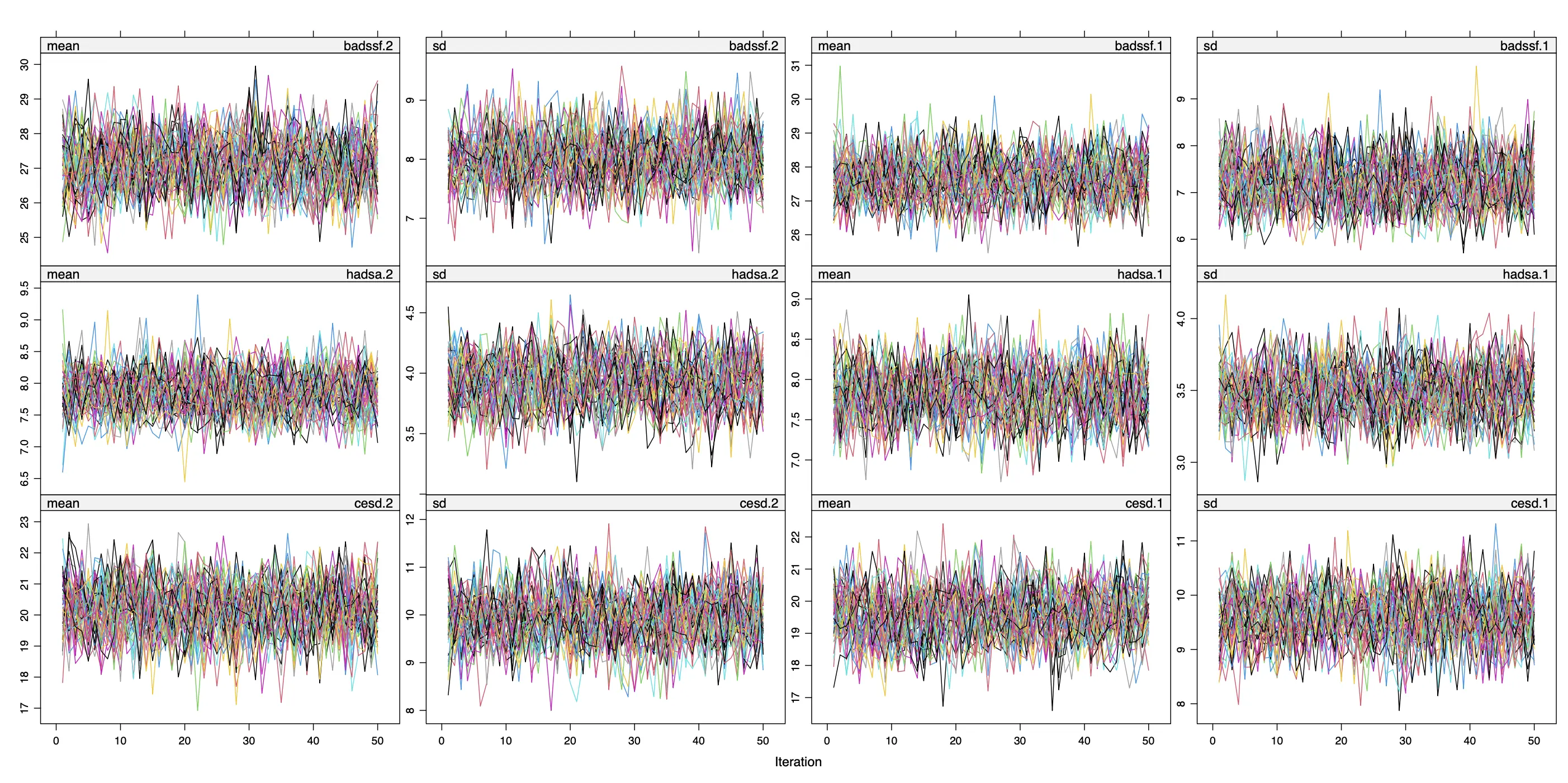
Next, it is important to check our imputations for potential problems. We want to confirm that, for all imputed variables, the MICE algorithm has converged to a stable solution. A good way to diagnose potential convergence issues is to generate a trace plot for all imputed variables:
The trace line plot shows, for all imputed variables, the mean and standard deviation of the imputed values \(\dot{\mathbf{Y}}_{\textsf{mis}}\) on the \(y\)-axis, while the \(x\)-axis shows the specific MICE iteration at which this value was obtained. Since we generated \(m\)=50 imputation sets, 50 lines are shown in each plot.
If the algorithm has converged, our imputed values should hover randomly around some specific value, with no particular trend visible over time. Furthermore, we also want that all trace lines are properly mixed and no imputation set displays consistently higher or lower values than others.
A good metaphor, as mentioned by Lunn and colleagues (2012, chap. 4.4.1), is that the trace lines should appear like a “fat hairy caterpillar”. This is arguably the case in our example, which increases our confidence that the imputations are usable for further analyses.
Examples of Non-Convergence
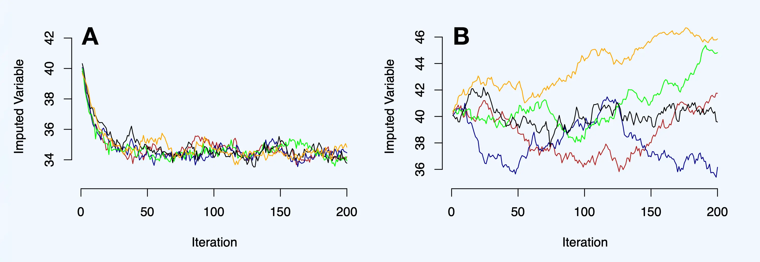
Given that the trace lines in our example above behaved quite “orderly”, we also simulated examples in which this is not the case (cf. van Buuren 2018, chap. 4.5.7)
Panel A below displays slow convergence, which can sometimes occur if the number of missings is very large. As we can see, the imputed values display a clear downward trend roughly until the 50th iteration; after that, the chains become stationary. In this scenario, the MICE algorithm does converge, but it is necessary to have a sufficient amount of iterations (approximately 50-100 in this case) before trustworthy estimates trickle through.
A much more troublesome case of actual non-convergence is displayed in panel B. In this scenario, even after 200 iterations, no clear stationarity is reached: the different trace lines scatter around without any visible pattern, and the chains do not mix either. Trace lines like this would be cause for concern but thankfully are rarely seen in practical applications.
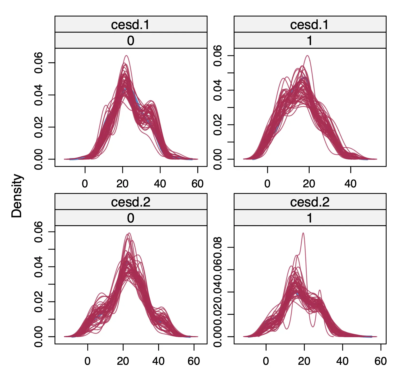
Another thing we can do to check our imputations is to create a density plot. The mice package has a special function called densityplot for this purpose. For now, we focus on inspecting the imputed value distributions in our primary outcome, the CES-D score at post-test and follow-up. The densityplot function also allows us to define a formula within the call, which can be used to generate separate plots for the intervention and control group:
These plots show, in red, the distribution of the imputed values for each of the 50 imputation sets. Looking closely, we also see the original distribution of observed outcomes, which is plotted in blue. Typically, a plausible imputation model should produce imputed values \(\dot{\mathbf{Y}}_{\textsf{mis}}\) that have a distribution similar to the one of \(\mathbf{Y}_{\textsf{obs}}\), as is the case here.
However, please note that under MAR, systematic differences in the distribution of \(\dot{\mathbf{Y}}_{\textsf{mis}}\) and \(\mathbf{Y}_{\textsf{obs}}\) are also plausible (e.g., differences in the mean or dispersion of values). It is extreme divergences or an excess of very unrealistic results that may point to potential problems with the imputation model. The distribution of imputed and observed values can also differ substantially when only a few values had to be imputed. If only, say, 3-4 values were imputed, this of course makes it much more likely that their density does not follow a bell-type shape like many of the red lines in our example above do.
3.2.3 Reference-Based Imputation
In the last section, ran our first imputation model using the MICE algorithm. As we mentioned before, these imputations were generated under the MAR assumption. We imputed values separately for the intervention and control group, assuming that the information recorded for both groups is sufficient to generate a valid approximation of the missing values.
The MAR assumption can be a plausible “first start” to handle missing outcomes, provided a sufficient amount of meaningful auxiliary variables is available. However, it is by no means guaranteed that the data are indeed MAR, and that our imputations are valid. Typically, it is not advisable to blindly trust that the MAR assumption will hold in our particular data set; instead, we should conduct sensitivity analyses that account for potential departures from MAR (Tan et al. 2021; Cro et al. 2020).
This means that additional imputation methods should be used that handle missing values under the MNAR assumption. This is a challenging task, since we do not know, and cannot prove, to which extent our missingness pattern is related to the missing values themselves.
Several techniques have been developed to handle MNAR data in the past. One example are selectionHeckman (1979) and pattern-mixture models(Thijs et al. 2002; Glynn, Laird, and Rubin 1986). These approaches add a shift parameter \(\delta\) to the imputed values, thus modeling the assumption that missing values differ systematically from the recorded ones. This allows us to, for example, model the assumption that patients with missing values had systematically worse outcomes at post-test, and that this is why they are missing. This adjustment requires one to assume a plausible value of \(\delta\), or a range thereof.
A related method that is sometimes used in pharmaceutical research is tipping point analysis, in which one studies how severely the missing values would have to differ from the observed ones to render the effect of an analysis non-significant (Liublinska and Rubin 2014).
A more recent method that lends itself particularly well to clinical trial evaluations is controlled multiple imputation, specifically the so-called reference-based imputation methods as described by Carpenter, Roger and Kenward (2013). The particular type of reference-based imputation that we will implement next in our own example trial uses the so-called jump-to-reference (J2R) approach (Carpenter, Roger, and Kenward 2013; I. White, Joseph, and Best 2020). So let us take some time to explain this method a little.
At first glance, the J2R approach closely resembles a MICE-based imputation under the MAR assumption. It selects a set of covariates from our data to impute missing values, and, like MICE, it is also an MI technique that generates multiply imputed data. After fitting the desired models in all data sets, estimates are then pooled into one result. This is often (but not always, J. W. Bartlett and Hughes 2020; J. W. Bartlett 2023) done using the same methods that are used for “conventional” MI.
Figure 3.1: Illustration of reference-based imputation (“jump-to-refence” approach).
The key distinction is that J2R relies on specific assumptions about the trajectory of patients’ outcomes starting from the point at which data are missing. The J2R approach assumes that, in terms of their outcomes, individuals in the intervention “jump” to the reference group (i.e., the control group) once they are lost to follow-up (see Figure 3.1). This assumption is very plausible in trials that do not include off-treatment assessments, as is often the case in pharmacological research. In such studies, individuals are not followed up anymore once they stop using the treatment; for example when they discontinue the medication under study.
Obviously, in this scenario, the missing outcome values are likely to differ systematically from the recorded ones: the patients who do not respond well, or experience negative side effects, are also the ones most likely to have missing outcomes. The J2R approach tries to account for this by imputing values as if the participant was now part of the control group. Thus the name “jump to reference”.
Computationally, this is typically done by fitting a Bayesian multivariate normal model with meaningful baseline covariates in both groups. Missing values of intervention group participants are then drawn from the distribution of the reference group to generate imputed values for each specific time point, and based on the participant’s baseline characteristics.
The J2R method offers a sensible method to impute missing values in trials without off-treatment assessments. In this case, it is often even used as the main imputation model. However, it may be less appropriate in other contexts. The J2R method essentially assumes that intervention participants lose all treatment benefits they may have experienced before being lost to follow-up. This is, arguably, quite an extreme position (Iddrisu and Gumedze 2019).
It is also unclear how sensible such an assumption is in, for example, psychological treatments, which typically do not have a clear-cut dose-response relationship (Robinson, Delgadillo, and Kellett 2020; Shalom and Aderka 2020). Furthermore, many trials at least try to obtain outcome assessments from the intervention group no matter if patients used the treatment as intended or not. This approach was also followed in our example trial. If a considerable amount of off-treatment assessments are available, this also strengthens the plausibility of an imputation under MAR.
Nevertheless, the J2R method might lend itself quite well to sensitivity analyses. This is because its assumptions are quite extreme. Analyzing J2R-imputed data allows us to obtain an estimate of the treatment effect under a plausible worst-case scenario in which we assume that all intervention participants who dropped out of our trial did so because the intervention was ineffective for them.
There are now several packages that allow to implement reference-based imputation in R, for example, rbmi(Gower-Page and Noci 2022) or mlmi(J. Bartlett 2021). However, the package we will be using here is RefBasedMI(McGrath 2023), which is based on the mimix program in STATA.
At the time we are writing this, the RefBasedMI package is not available on CRAN. That means that we need to install the package directly from its online repository. To do this, we have to install and load the remotes package (Csárdi et al. 2021) first, after which we can use the following code to install RefBasedMI.
Next, we have to reshape our trial data set to a format the RefBasedMI can work with. Currently, our data is in the wide format: each participant of the trial is represented by exactly one row. We now have to convert the data to the long format, where each participant has two rows: one for the post-test assessment, and another one with the 3-month follow-up scores.
Reshaping data frames in R is not an easy task, especially for beginners. Here we show code based on the pivot_longer function (which is included in the tidyverse) that can be used to bring our data into the desired format. Please note that this approach is “re-usable” for other trial data sets too, as long as the same coding guidelines are followed.
First, we have to create a new numeric id variable in our data set, like so:
data$id <-1:nrow(data)
Next, we use the pivot_longer function to reshape our data into the desired long format. We save the results as data.long.
The reshaping creates a new variable in our data set called time, which encodes the post-randomization measurement point at which a value was obtained. We can examine this variable a little further:
We can see that the value of this variable is either "1" or "2", indicating if the value was obtained at post-test or 3-month follow-up. Using the mutate function, we now recode the two values to 7 and 12, respectively, indicating the actual number of weeks after randomization at which participants were assessed.
We see that, for each of our outcomes assessed after randomization (badssf, hadsa, cesd), the data frame now provides values for the post-test measurement (time=7) and follow-up (time=12) in the value column. Importantly, note that the baseline measurement of, e.g., the CES-D is included as a separate column (cesd.0), which has the same value across all measurement points and outcomes for each participant.
The reference-based imputation method implemented in RefBasedMI is less flexible than mice. For example, it is necessary that all co-variates that we want to include in the imputation model are completely recorded. Furthermore, reference-based imputations can only be generated for one outcome at a time, which means that we have to run the function separately for the CES-D, BADS-SF and HADS-A values.
Since we use J2R as a sensitivity analysis in this example, we only focus on our primary outcome for now, the CES-D values. This means that we can filter out all cesd measurements using the outcome variable. We save the resulting data frame as data.long.cesd.
In the covar argument, we can specify the baseline variables conditional on which imputations should be generated. Here, we use the same baseline variables as were included in the predictor matrix when using MICE (see Section 3.2.2).
2
The depvar argument can be used to specify the outcome variable we want to impute; in our case, this is the value column.
3
The treatvar, idvar and timevar arguments specify the treatment, ID and assessment point variable, respectively.
4
In the method argument, we specify the imputation approach we want to apply. Several options are available, for example "MAR" for a “simple” MAR imputation, "CR" for “copy reference”, which is another type of reference-based imputation; or "J2R", which implements the J2R approach we want to use for our example.
5
In the reference argument, we have to specify the value of the group variable provided in treatvar that corresponds with the reference/control group. In our case, this is 0, since this value has been used for participants in the waitlist control group.
6
The M argument controls the number of imputation sets that are generated (\(m\)=50 in our case), while the seed argument can be used to set a random number generator seed.
7
After that, we use the as.mids function in a pipe to convert the results to a mids object. This is helpful because this is the same type of object that is also created by mice, which means that the resulting multiply imputed datasets can be analyzed in the same way.
8
We save the result as imp.j2r.
This implementation should be faster than mice, with imputations generated within 1-2 minutes. It is advisable to save the imputed data right away as an .rda file:
save(imp.j2r, file="imp.j2r.rda")
Congeniality of the Imputation & Analysis Model
Introduced by Meng (1994), the term congeniality refers to the idea that our imputation and analysis model should be “of the same kind”. One of the advantages of MI is that it allows us to analyze our data using the same model we would have used if all data had been observed; this is also known as the substantive analysis model.
Congeniality means that the assumptions we make in our imputation model should be compatible with what we assume about our data in the substantive analysis model. For this reason, congeniality is also sometimes referred to as substantive model compatibility(J. W. Bartlett et al. 2015; Quartagno and Carpenter 2022b).
One example of this are clustered data (e.g. individual participant data from several studies, or multi-centre RCT data). In this case, a multilevel imputation model has to be used, because the substantive analysis model also assumes a clustered data structure (e.g. if we used mixed-effects or IPD meta-analytic models); otherwise, estimates that we obtain from the model may not be valid. A package that is designed particularly for multilevel imputation models is mitml(Grund, Robitzsch, and Luedtke 2021). However, this package can also be helpful when the data are not clustered, and we will use some of its functionality later in this tutorial.
There are now several packages in R that implement so-called substantive model compatible multiple imputation (SMC-MI), which ensures that the imputations are strictly compatible with the substantive analysis model we want to apply in the next step; for example the smcfcs package (which uses an FCS-based approach, J. Bartlett, Keogh, and Bonneville 2022), or the JointAI package (which uses a joint Bayesian approach in which data are imputed and analyzed in one step, Erler, Rizopoulos, and Lesaffre 2021). These implementations may be beneficial if our substantive analysis model assumes, e.g., complex interactions or non-linear relationships.
3.3 Rubin’s Combination Rules
After having generated our multiply imputed data, we can now proceed to the next step, in which our analysis model is fitted in each data set and then pooled. This adds another level of complexity: when the same analysis is conducted in \(m\) data sets simultaneously, this also means that we obtain \(m\) results, which differ more or less from each other due to our imputation uncertainty. Our goal, however, is to come up with one result (e.g. one estimate of the mean difference between groups, and whether this difference is significant) that we and others can interpret. To generate such a pooled result across all imputed data sets, we use a set of formulas that are commonly known as Rubin’s Rules in the literature (Rubin 2004; Barnard and Rubin 1999; van Buuren 2018, chaps. 2.4, 5.2).
Rubin’s combination rules take into account that all estimates we can obtain from our data are subject to uncertainty. In the case of multiply imputed data, there are two reasons for this:
Participants in our trial are only a sample from a much greater population that we want to study, which means that some degree of sampling error can be expected.
Our data contain missing values that had to be imputed. We do not know the true value of these imputations, which means that they also make our estimates less certain. This uncertainty is reflected by the fact that multiply imputed values may differ slightly between imputation sets.
In essence, the goal of Rubin’s rules is to generate pooled estimates (and, even more important, confidence intervals around them) that properly integrate these two sources of variation. It allows to obtain results that reflect both our uncertainty due to sampling error, which occurs even if all data had been recorded and the additional uncertainty due to the fact that some of our data are mere imputations; not “real” values that we know for sure.
Let us introduce some notation. Let \(Q\) be a true value (or a vector of true values) in the population that we want to estimate (e.g. a population mean, regression coefficient, or the like). Due to the reasons we named above, \(Q\) is unknown and must be approximated by an estimate thereof, \(\hat{Q}\). This is only possible using the observed values \(Y_{\textsf{obs}}\). The expected value \(\mathbb{E}\), the best possible approximation of \(Q\) given our observed values \(Y_{\textsf{obs}}\) is (van Buuren 2018, chap. 2.3.2):
This formula looks very abstract and complex, but it helps to read it from the outside to the inside. It tells us that the best approximation of \(Q\) given \(Y_{\textsf{obs}}\) is to take the expected value of the expected values in all imputed data sets. Let us make this more concrete: if \(Q\) is, for example, a population mean, we can take the average of all the means calculated in each of our multiply imputed data sets to obtain the best possible approximation given our data. We can also formalize this. Let \(\hat{Q}_\ell\) be the estimate of \(Q\) in some imputation set \(\ell\), where \(m\) is the total number of imputation sets we generated. The “pooled” estimate of \(Q\) is thus:
This formula can be used in practice to obtain a pooled point estimate within our multiply imputed data: we calculate the value of the point estimate (e.g., a sample mean or regression weight) in each imputed data set individually, and then take the average of these calculated values across all imputation sets. Please note that this simple aggregation method cannot be used if we want to pool test statistics (e.g. \(t\) or \(F\) values), and it is also not advisable if we want to combine correlations. We will cover how to deal with such estimates later in this chapter.
Naturally, we are not only interested in point estimates but also in their uncertainty. To calculate \(P\) values and confidence intervals around our estimates, we also need to calculate the pooled variance of \(Q\) in our multiply imputed data. Here, we cannot simply analyze all data sets as if they would contain no missings and then average the results. As mentioned before, we have to take into account that there are two sources of variation that determine the uncertainty of our estimate:
\[
\mathrm{Var}[Q|Y_{\textsf{obs}}] = \underbrace{\mathbb{E}\bigg[\mathrm{Var}[Q|Y_{\textsf{obs}}, Y_{\textsf{mis}}]~ \bigg| ~ Y_{\textsf{obs}} \bigg]}_{\scriptsize \begin{split} &\textsf{mean of the variances across MI sets} \\ & {\rightarrow \textbf{Within-Variance}~(\bar{{U}})} \end{split}} + \underbrace{\mathrm{Var}\bigg[ \mathbb{E}[Q|Y_{\textsf{obs}}, Y_{\textsf{mis}}]~\bigg|~ Y_{\textsf{obs}}\bigg]}_{\scriptsize \begin{split} &\textsf{variance of the means across MI sets} \\ & {\rightarrow \textbf{Between-Variance}~(B)} \end{split}}
\tag{3.13}\]
As shown in the equation above, these two components are the “general” variance \(\bar U\) that we find within each imputed data set, and the variation \(B\) of our estimate of \(Q\)between imputation sets. These components coincide with the two sources of variation we discussed before: \(\bar U\) represents the (averaged) variance due to sampling error, while \(B\) is the variation due to imputation uncertainty. In practice, the pooled variance \(\hat V\) can be calculated using Rubin’s rules:
It is not essential to understand every detail of this equation. The core part is indicated by the braces, which shows that using Rubin’s rules, we combine the within-variance \(\bar U\) and between variance \(B\) to obtain the correct estimate of our total variance \(\hat V\). The parts of the equation displayed in blue show a third source of variation: in practice, we can only generate a finite amount of imputation sets \(m\), and this simulation variance adds another source of uncertainty that is accounted for in the formula.
The equation above also shows that, as \(m\) goes to infinity, this variation source drops out of the equation, leaving only the \(\bar U\) and \(B\) components that we discussed before. This part of the Rubin formula is one of the reasons why it is sensible to have a larger number of imputed data sets since this means that the term \((1+1/m)\) becomes smaller. Especially when very accurate variance estimates are necessary, a high number of imputation sets is therefore recommended. A low \(m\) leads to confidence intervals that are slightly wider than when \(m \rightarrow \infty\) (statisticians call this lower efficiency). However, this difference is typically manageable in practice.
3.3.1 Metrics for Parameter Estimates in MI
There are a few metrics that can be derived from the estimate of the within- and between-variance \(\bar U\) and \(B\). These metrics allow us to better understand the extent to which missing data has impacted the uncertainty of our pooled results. One of these metrics is the relative increase in variance due to non-response, or RIV, which quantifies the amount of between-imputation variation of \(Q\) in relation to the “real” variance in our imputed variable. It is calculated like this:
Whereby values of \(r_Q >\) 1 indicate that the imputation variance is greater than the average within-variance in our data.
Another metric is the fraction of missing information due to non-response (FMI). This is the fraction of information about \(Q\) that was “lost” due to our imputation uncertainty. It is calculated using the following formula:
Where \(r_Q\) is the RIV from above, and \(\nu_Q\) (nu) are the degrees of freedom in the estimation of \(Q\). There is a special way in which these degrees of freedom are calculated in analyses of multiply imputed data, as we will see in the next section.
3.3.2 Degrees of Freedom in MI Analyses
The degrees of freedom of a model are typically defined as the number of observations minus the number of model parameters: \(\nu = n - k\) (e.g., for the mean: \(\nu = n - 1\)). With MI, some elements of \(n\) are only estimates of observations that were not recorded, which means that \(\nu\) also has to be corrected accordingly for this:
Where \(r\) is the relative increase in variance we discussed in the previous chapter. This formula has a special property that we see when setting \(r\), the RIV, to zero. When \(r=0\), this means that all data has been recorded and that there has been no increase in variance due to non-response. In this scenario, the value of \(\nu_{(MI)}\) returned by the formula is infinity:
Put differently, the formula works under the assumption that the degrees of freedom of the complete data model are infinitely large. This large-sample approximation is only sensible when our sample is relatively big.
For small samples, an adapted formula needs to be used (Barnard and Rubin 1999). This requires us to first determine the “hypothetical” degrees of freedom of our model if our data had been fully recorded. We call this the complete data degrees of freedom, \(\nu_{\textsf{com}}\), which are calculated from the number of observations \(n\) and parameter number \(k\):
\[
\nu_{\textsf{com}} = n-k
\tag{3.19}\]
This way, we can determine the degrees of freedom of the observed values, \(\nu_{\textsf{obs}}\):
The unadjusted degrees of freedom formula is the default used by the mitml package that we will be using in our analysis later on. Please note that, if this formula is used, the degrees of freedom of a parameter can be larger than the total number of observations \(n\). Also, since the degrees of freedom are merely approximated by the formulas above, the value of \(\nu\) also does not have to be a natural number (values like, e.g., \(\nu =\) 256.5669 are also perfectly possible).
3.3.3 MI-Based Confidence Intervals
The calculated degrees of freedom can be used to construct a confidence interval around our point estimate. For the inference of scalars (i.e., when \(\bar Q\) is a single value), a \(t\)-distribution is typically assumed. The \(t\)-value is determined based on the reference value of our null hypothesis \(Q_0\), which is usually 0:
Whereby the test of \(t\) depends on the degrees of freedom \(\nu\). Using the calculated MI degrees of freedom \(\nu_{\textsf{(MI)}}\), we can then calculate a confidence interval around \(\bar Q\) that accounts for our imputation uncertainty:
The mitml package that we will be using in this analysis contains functions that allow constructing such confidence intervals directly for us.
3.3.4 Analysis of MI Data: Caveats & Special Cases
Before we complete this chapter, we want to cover a few special cases and caveats to keep in mind when pooling the results obtained from multiply imputed data.
Our first point pertains to the aggregation of test statistics, such \(t\), \(\chi^2\), or \(F\) values obtained by some model. Such test statistics are often calculated in practice, but it is not possible to simply pool them using the arithmetic mean, as we did with \(\bar Q\). The reason for this is that the value of a test statistic depends on the variance and degrees of freedom of our model. However, as we learned, when some missing values had to be imputed, the overall variance increases because imputation uncertainty is added to our estimates.
Thus, the pooled value of the test statistic also needs to reflect this. To avoid overestimating test statistics, special aggregation formulas must be used. Luckily, there are now several implementations in R that can do this for us, such as the micombine.chisquare and micombine.F functions in miceadds. In our hands-on analysis, we will showcase how to implement these functions in practice.
Another special case in MI analyses are correlations. The value of a correlation \(\rho\) cannot exceed the maximum values \([-1;1]\). This means that the variance of \(\rho\) is restricted the closer \(\rho\) gets to 1 or -1. As a result, we cannot assume that \(\rho\) is asymptotically normal. Thus, to aggregate correlations, it is not advisable to simply calculate the mean of all correlations we obtained in the multiply imputed data. Instead, we should first apply a variance-stabilizing transformation by calculating what is known as Fisher’s \(z\). In R, such a transformation is applied automatically if we use the micombine.cor function, which is also part of the miceadds package.
Aggregating MI Sets
Lastly, we also want to bring attention to a commonly used, but generally inappropriate approach to dealing with multiply imputed data. In practice, it is often seen that analysts aggregate all MI sets into one data set without missings, and then proceed to conduct their analyses in this single data set. Naturally, this makes an analysis using conventional statistical software a lot easier; but this approach should definitely be avoided from a statistical perspective. Aggregating into one dataset “pretends” that there is no imputation uncertainty; this leads to incorrect (that is, anti-conservative) \(P\) values, confidence intervals, test statistics, and so forth. An analysis of aggregated data should only be performed if no statistical tests or quantification of parameter uncertainty is needed. Yet, this is rarely the case in practice.
3.4 Functional Programming
The last chapter was quite theoretical, and we can assure you that things will become more hands-on from now on. In this section, we will cover a more practical issue in the analysis of multiply imputed data, and how we can solve it using R.
As we have learned, an appropriate analysis of MI data requires us to fit the desired analysis not only once, but in each of the \(m\) generated data sets in parallel. This is easier said than done. If we want to perform some operation in several data sets at the same time, even presumably easy analysis steps can become markedly more complex.
To illustrate this, let us go back to our imp object that we created in Section 3.2.2. This object contains the multiply imputed data that we generated using MICE. As a next step, we use the mids2mitml.list function in the mitml package to convert this object to a simple list, in which each list element contains one of the imputed sets. We save the result as implist.
library(mitml)implist <-mids2mitml.list(imp)
How can we analyze all the imputed data sets in this list simultaneously? Imagine that, for example, we want to calculate the mean of our primary outcome variable cesd.1 in all data sets, and then average them to get a pooled estimate. A commonly used approach is to use a for loop for this purpose. This allows us to go through each list element (viz., imputed data set) one after another, calculate the mean, and save it in a new variable that we will call means here. After that, we can take the average of means to obtain our final result.
1means <-vector()2for (i in1:50){ means[i] <- implist[[i]] %>%pull(cesd.1) %>%mean()}3mean(means)
1
Create an empty vector in which our results will be stored.
2
Loop through all \(m\)=50 imputation sets.
3
Calculate the mean value across imputation sets.
Show result
## [1] 19.77795
Do not worry if you have never heard of for loops before, or if you do not understand everything about the code that we used here. The example above only goes to show that a rather straightforward operation (taking the mean of a variable) can become tricky when we have to apply it in all data sets simultaneously. The code above is quite complex. Furthermore, if we had performed a more involved analysis than simply extracting the mean, we would have also seen that this approach can lead to quite long computation times.
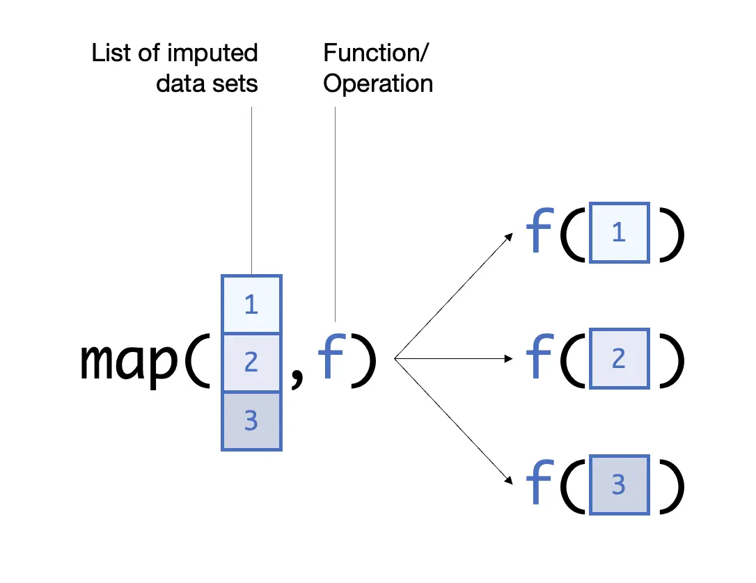
A better approach to perform operations in multiply imputed data is to use functional programming. In a functional programming approach, we use a single function that applies some operation to all imputation sets for us at the same time. Base R contains functions like apply, mapply, vapply, or Reduce to do this. However, a particularly user-friendly and broadly applicable option are the map functions included in the purrr package (Henry and Wickham 2020). To illustrate this, here is how we can apply the same operation from before using map:
implist %>%map_dbl(~mean(.$cesd.1)) %>%mean()
This code is less convoluted than our for loop, and it also runs faster.
In essence, every call to map requires two arguments: a list object in which each element contains a different imputation set, as well as the function we want to apply in each of these elements. Once we run the function, map will then automatically apply the defined operation in each set and provide us with a list of the results.
The inner workings of map.
The map function comes in different “flavors”, depending on the type of object that should be returned. The map_dbl, map_chr, map_lgl and map_dfr functions can be used depending on whether we want the results to be a numeric, character or logical vector, or a data frame, respectively. In all of the map functions, the second argument specifies the type of function that should be performed in all list elements. There are two ways to specify this function; the first is to supply a “fully functioning” (no pun intended) function. This function has exactly one argument x, whereby x represents one individual list element. Here is an example:
# 'x' represents the individual list element in 'list'map(list, function(x) mean(x$variable))
The other option is to use a shortened notation, in which we use a tilde (~) to indicate the start of the function, and a dot (.) to represent the individual list element. Here is the same example from above using this shortened notation:
# '.' represents the individual list element in 'list'map(list, ~mean(.$variable))
It typically requires a little practice until one becomes fully familiar with functional programming as implemented in map. Nonetheless, it is worth the effort: analyses of multiply imputed data require us to apply functions in lists of data sets all the time, which makes map an indispensable tool in practice.
\(\blacksquare\)
Barnard, John, and Donald B Rubin. 1999. “Miscellanea. Small-Sample Degrees of Freedom with Multiple Imputation.”Biometrika 86 (4): 948–55. https://doi.org/10.1093/biomet/86.4.948.
Bartlett, Jonathan W. 2023. “Reference-Based Multiple Imputation—What Is the Right Variance and How to Estimate It.”Statistics in Biopharmaceutical Research 15 (1): 178–86. https://doi.org/10.1080/19466315.2021.1983455.
Bartlett, Jonathan W, and Rachael A Hughes. 2020. “Bootstrap Inference for Multiple Imputation Under Uncongeniality and Misspecification.”Statistical Methods in Medical Research 29 (12): 3533–46. https://doi.org/10.1177/0962280220932189.
Bartlett, Jonathan W, Shaun R Seaman, Ian R White, James R Carpenter, and Alzheimer’s Disease Neuroimaging Initiative. 2015. “Multiple Imputation of Covariates by Fully Conditional Specification: Accommodating the Substantive Model.”Statistical Methods in Medical Research 24 (4): 462–87. https://doi.org/10.1177/0962280214521348.
Bartlett, Jonathan, Ruth Keogh, and Edouard F. Bonneville. 2022. smcfcs: Multiple Imputation of Covariates by Substantive Model Compatible Fully Conditional Specification. https://CRAN.R-project.org/package=smcfcs.
Bell, Melanie L, Mallorie Fiero, Nicholas J Horton, and Chiu-Hsieh Hsu. 2014. “Handling Missing Data in RCTs; a Review of the Top Medical Journals.”BMC Medical Research Methodology 14 (1): 1–8. https://doi.org/10.1186/1471-2288-14-118.
Bell, Melanie L, Michael G Kenward, Diane L Fairclough, and Nicholas J Horton. 2013. “Differential Dropout and Bias in Randomised Controlled Trials: When It Matters and When It May Not.”BMJ 346. https://doi.org/10.1136/bmj.e8668.
Carpenter, James R, James H Roger, and Michael G Kenward. 2013. “Analysis of Longitudinal Trials with Protocol Deviation: A Framework for Relevant, Accessible Assumptions, and Inference via Multiple Imputation.”Journal of Biopharmaceutical Statistics 23 (6): 1352–71. https://doi.org/10.1080/10543406.2013.834911.
Carpenter, James R, and Melanie Smuk. 2021. “Missing Data: A Statistical Framework for Practice.”Biometrical Journal 63 (5): 915–47. https://doi.org/10.1002/bimj.202000196.
Cro, Suzie, Tim P Morris, Michael G Kenward, and James R Carpenter. 2020. “Sensitivity Analysis for Clinical Trials with Missing Continuous Outcome Data Using Controlled Multiple Imputation: A Practical Guide.”Statistics in Medicine 39 (21): 2815–42. https://doi.org/10.1002/sim.8569.
Csárdi, Gábor, Jim Hester, Hadley Wickham, Winston Chang, Martin Morgan, and Dan Tenenbaum. 2021. remotes: R Package Installation from Remote Repositories, Including GitHub. https://CRAN.R-project.org/package=remotes.
de Silva, Anurika Priyanjali, Margarita Moreno-Betancur, Alysha Madhu de Livera, Katherine Jane Lee, and Julie Anne Simpson. 2017. “A Comparison of Multiple Imputation Methods for Handling Missing Values in Longitudinal Data in the Presence of a Time-Varying Covariate with a Non-Linear Association with Time: A Simulation Study.”BMC Medical Research Methodology 17: 1–11. https://doi.org/10.1186/s12874-017-0372-y.
Enders, C K. 2010. Applied Missing Data Analysis. 1st ed. New York City: Guilford Publications.
Enders, Craig K, Timothy Hayes, and Han Du. 2018. “A Comparison of Multilevel Imputation Schemes for Random Coefficient Models: Fully Conditional Specification and Joint Model Imputation with Random Covariance Matrices.”Multivariate Behavioral Research 53 (5): 695–713. https://doi.org/10.1080/00273171.2018.1477040.
Erler, Nicole S., Dimitris Rizopoulos, and Emmanuel M. E. H. Lesaffre. 2021. “JointAI: Joint Analysis and Imputation of Incomplete Data in R.”Journal of Statistical Software 100 (20): 1–56. https://doi.org/10.18637/jss.v100.i20.
Glynn, Robert J., Nan M. Laird, and Donald B. Rubin. 1986. “Selection Modeling Versus Mixture Modeling with Nonignorable Nonresponse.” In Drawing Inferences from Self-Selected Samples, edited by Howard Wainer, 115–42. New York, NY: Springer. https://doi.org/10.1007/978-1-4612-4976-4_10.
Grund, Simon, Oliver Lüdtke, and Alexander Robitzsch. 2018. “Multiple Imputation of Missing Data at Level 2: A Comparison of Fully Conditional and Joint Modeling in Multilevel Designs.”Journal of Educational and Behavioral Statistics 43 (3): 316–53. https://doi.org/10.3102/1076998617738087.
Grund, Simon, Alexander Robitzsch, and Oliver Luedtke. 2021. mitml: Tools for Multiple Imputation in Multilevel Modeling. https://CRAN.R-project.org/package=mitml.
Heckman, James J. 1979. “Sample Selection Bias as a Specification Error.”Econometrica 47 (1): 153–61. https://doi.org/10.2307/1912352.
Iddrisu, Abdul-Karim, and Freedom Gumedze. 2019. “An Application of a Pattern-Mixture Model with Multiple Imputation for the Analysis of Longitudinal Trials with Protocol Deviations.”BMC Medical Research Methodology 19: 1–23. https://doi.org/10.1186/s12874-018-0639-y.
Little, Roderick J A. 1988. “A Test of Missing Completely at Random for Multivariate Data with Missing Values.”Journal of the American Statistical Association 83 (404): 1198–1202. https://doi.org/10.2307/2290157.
Liublinska, Victoria, and Donald B Rubin. 2014. “Sensitivity Analysis for a Partially Missing Binary Outcome in a Two-Arm Randomized Clinical Trial.”Statistics in Medicine 33 (24): 4170–85. https://doi.org/10.1002/sim.6197.
Lunn, David, Christopher Jackson, Nicky Best, Andrew Thomas, and David Spiegelhalter. 2012. The BUGS Book. A Practical Introduction to Bayesian Analysis. 1st ed. Chapman Hall.
McGrath, Kevin. 2023. RefBasedMI: Reference-Based Imputation for Longitudinal Clinical Trials with Protocol Deviation. https://github.com/UCL/RefBasedMI.
Meng, Xiao-Li. 1994. “Multiple-Imputation Inferences with Uncongenial Sources of Input.”Statistical Science 9 (4): 538–58. https://doi.org/10.1214/ss/1177010269.
Molenberghs, Geert, Herbert Thijs, Ivy Jansen, Caroline Beunckens, Michael G Kenward, Craig Mallinckrodt, and Raymond J Carroll. 2004. “Analyzing Incomplete Longitudinal Clinical Trial Data.”Biostatistics 5 (3): 445–64. https://doi.org/10.1093/biostatistics/5.3.445.
Morris, Tim P, Ian R White, and Patrick Royston. 2014. “Tuning Multiple Imputation by Predictive Mean Matching and Local Residual Draws.”BMC Medical Research Methodology 14: 1–13. https://doi.org/10.1186/1471-2288-14-75.
Quartagno, Matteo, and James R Carpenter. 2022b. “Substantive Model Compatible Multilevel Multiple Imputation: A Joint Modeling Approach.”Statistics in Medicine 41 (25): 5000–5015. https://doi.org/10.1002/sim.9549.
Quartagno, Matteo, Simon Grund, and James Carpenter. 2019. “jomo: A Flexible Package for Two-Level Joint Modelling Multiple Imputation.”The R Journal 11 (2): 205–28. https://doi.org/10.32614/RJ-2019-028.
Robinson, Louisa, Jaime Delgadillo, and Stephen Kellett. 2020. “The Dose-Response Effect in Routinely Delivered Psychological Therapies: A Systematic Review.”Psychotherapy Research 30 (1): 79–96. https://doi.org/10.1080/10503307.2019.1566676.
Shalom, Jonathan G, and Idan M Aderka. 2020. “A Meta-Analysis of Sudden Gains in Psychotherapy: Outcome and Moderators.”Clinical Psychology Review 76: 101827. https://doi.org/10.1016/j.cpr.2020.101827.
Tan, Ping-Tee, Suzie Cro, Eleanor van Vogt, Matyas Szigeti, and Victoria R Cornelius. 2021. “A Review of the Use of Controlled Multiple Imputation in Randomised Controlled Trials with Missing Outcome Data.”BMC Medical Research Methodology 21 (1): 1–17. https://doi.org/10.1186/s12874-021-01261-6.
Thijs, Herbert, Geert Molenberghs, Bart Michiels, Geert Verbeke, and Desmond Curran. 2002. “Strategies to Fit Pattern-Mixture Models.”Biostatistics 3 (2): 245–65. https://doi.org/10.1093/biostatistics/3.2.245.
Thoemmes, F, and C K Enders. 2007. “A Structural Equation Model for Testing Whether Data Are Missing Completely at Random.” In Annual Meeting of the American Educational Research Association, Chicago, IL.
van Buuren, Stef. 2007. “Multiple Imputation of Discrete and Continuous Data by Fully Conditional Specification.”Statistical Methods in Medical Research 16 (3): 219–42. https://doi.org/10.1177/0962280206074463.
van Buuren, Stef, Jaap PL Brand, Catharina GM Groothuis-Oudshoorn, and Donald B Rubin. 2006. “Fully Conditional Specification in Multivariate Imputation.”Journal of Statistical Computation and Simulation 76 (12): 1049–64. https://doi.org/10.1080/10629360600810434.
van Buuren, Stef, and Karin Groothuis-Oudshoorn. 2011a. “mice: Multivariate Imputation by Chained Equations in R.”Journal of Statistical Software 45: 1–67. https://doi.org/10.18637/jss.v045.i03.
———. 2011b. “mice: Multivariate Imputation by Chained Equations in R.”Journal of Statistical Software 45 (3): 1–67. https://doi.org/10.18637/jss.v045.i03.
White, Ian R, Patrick Royston, and Angela M Wood. 2011b. “Multiple Imputation Using Chained Equations: Issues and Guidance for Practice.”Statistics in Medicine 30 (4): 377–99. https://doi.org/10.1002/sim.4067.
———. 2011a. “Multiple Imputation Using Chained Equations: Issues and Guidance for Practice.”Statistics in Medicine 30 (4): 377–99. https://doi.org/10.1002/sim.4067.
White, Ian, Royes Joseph, and Nicky Best. 2020. “A Causal Modelling Framework for Reference-Based Imputation and Tipping Point Analysis in Clinical Trials with Quantitative Outcome.”Journal of Biopharmaceutical Statistics 30 (2): 334–50. https://doi.org/10.1080/10543406.2019.1684308.
e.g., when there are considerably more missings in the intervention group than in the control group, as is often the case in mental health care research.↩︎