Show result
## [1] 3
In this section, we will be discussing all the steps that are required to set up your computer for the analyses we present in this tutorial. In particular, we will be introducing the statistical programming language R, the technicalities of which can often serve as a first obstacle for aspiring RCT analysts.
For many mental health researchers, working with R represents the first-ever exposure to a programming language, and we will cover what distinguishes R from Graphical User Interface (GUI)-based statistical software, which is still frequently used in practice. While this is sometimes exaggerated, R does indeed have a steep learning curve and requires continuous practice to become proficient in. While it is not possible to provide an in-depth introduction into R, we will describe how to set up an R environment on a personal computer and cover some fundamental operations that are needed on a day-to-day basis.
If you are an experienced R user, most of the following information will be nothing new and this section can therefore be skipped. Nevertheless, it might be helpful to go through this section anyway as a brief refresher.
R, like any programming language, has to be actively learned and used to become an expert. Frustration is a natural part of this process. Especially in the beginning, R might often feel unnecessarily cumbersome, especially if users are already accustomed to working with more “user-friendly” GUI-based software.
We all know that the greatest part of an iceberg lies below the water’s surface. Likewise, when learning R, it can take some time and practice until one sees the progress one has made. Learning R is still worth the effort: it provides us with arguably the most comprehensive, commonly used, and up-to-date statistical toolbox for our RCT analyses to date; and it is completely open-source and free.

To begin this tutorial, we first have to install the right version of R for our operating system (i.e., Windows or Mac). R comes in different versions, and it is advisable to always install the latest version. At the time we are writing this, the latest version of R is 4.2.2.
Besides R, we also install a so-called integrated development environment (IDE). IDEs are essentially computer programs that make working with programming languages like R more convenient. One of the best options for R specifically is RStudio, which can be downloaded here. Posit, the company behind RStudio, also offers a professional version but installing the free version is more than sufficient. RStudio is helpful because it is designed specifically for R. It makes it easier to write and execute code, as well as handle data, packages, and outputs.
R and RStudio are not identical: RStudio simply makes working with R easier; to use RStudio, R has to be already installed on our computer.
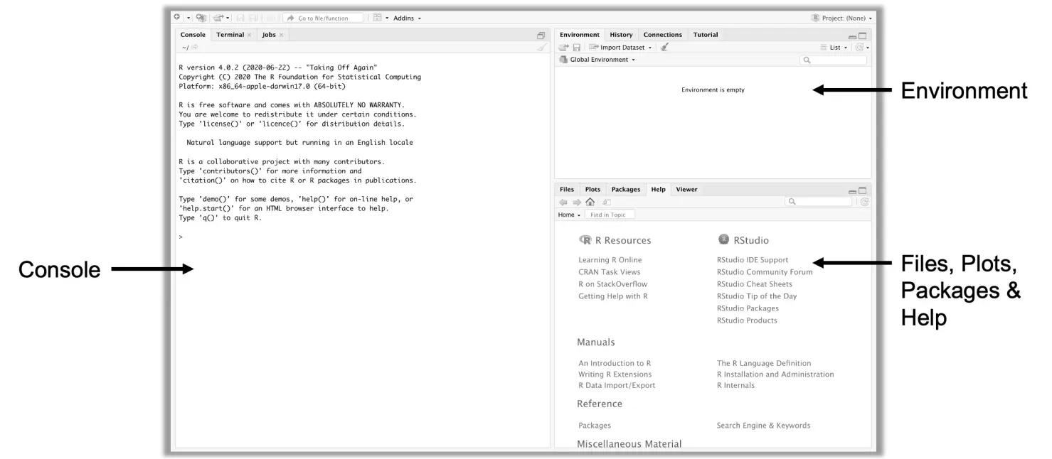
When opening RStudio, we are presented with a window with three panes:
A fourth pane, the editor, opens when a new R file is created (by clicking, in the toolbar on top, on “File” > “New File” > “R Script”). R scripts in the editor can be used to store important code. The scripts can be saved later via “File” > “Save” in a file with the extension _.R} on the computer.
R code is always executed in the console, and the editor is only used to write and store code. To execute code in the editor, we must pass it to the console. To do this, we have to select the relevant code chunk with our mouse, and then either hit \(\triangleright\) Run in the upper right corner of the editor or the key combination Ctrl/ Cmd + Enter.
One of the great strengths of R is that it provides functionality for almost any statistical method imaginable. In contrast to much other software, R is not restricted to the functions and tools that its developers originally created for it. Being a full programming language, experts all around the world can write extensions for R, so-called packages.
Packages represent a collection of R functions that may be useful for a particular problem or application. For example, the package The ggplot2 package (Wickham 2016) provides functions for creating graphs. Packages can be developed by experts around the world and then downloaded and used in R by anyone. The Comprehensive R Archive Network (CRAN) alone currently lists more than 16000 installable packages.
Some functions, operators, data sets, and plotting tools are already “pre-installed” in R. Many of these functions have existed since R was first developed in the early 1990s. These functionalities are collectively referred to as Base R and can be used without having to install additional packages. Some packages, such as stats or MASS (Venables and Ripley 2002), are also automatically installed with the first installation of R, and are therefore considered “Base R” too.
Besides Base R, there is the so-called tidyverse (Wickham et al. 2019). This is a selection of packages, all newer than Base R, which aim to simplify the manipulation and visualization of data using R. Three examples (two of which we also use later in our hands-on analysis) are:
ggplot2: A package to generate various types of graphs and visualizations. The package can also create highly advanced visualizations, as showcased by the . However, in this tutorial, we will keep things simple and only use the plotting tools that are already pre-installed in R (see e.g. Chapter ).dplyr: A package that contains helpful tools to manipulate data. Some basic familiarity with this package is highly recommended because it makes working with imported data (including RCT data) using R much more convenient. We will cover a few helpful functions included in dplyr in the next sections.purrr. A package to easily implement functional programming in R. This package is particularly helpful when we have to work with multiple versions of a data set at the same time, which is a common problem in RCT analyses that employ multiple imputation. Later in this text, we will discuss the core functions of this package in greater detail.Packages of the tidyverse are widely used in the R community and are particularly beginner-friendly. Therefore, the tidyverse is the first package we will be installing in this tutorial.
The Comprehensive R Archive Network, or CRAN, is an online package repository maintained by the R Foundation. CRAN hosts the bulk of R packages we need on a daily basis, which we can install on our own computer using the install.packages function. To let CRAN know which package we want to have installed on our computer, we have to provide its name in brackets. In our case, the first function we have to execute using R is:
install.packages("tidyverse")In other words, we have to type in the code above in the Console and then hit Enter. Please also note that R is case-sensitive, so please make sure that all letters in your call are lowercase, like in the box above. After hitting Enter, the console will print out information on the progress of the installation. Once the installation is complete, the tidyverse package will be added to your system library and will appear in the Packages pane, typically in the bottom-right of your RStudio window.
To be able to actually use functions included in a package, we have to load a package from the system library first. This is achieved using the library function:
library(tidyverse)Also note how, in the call to install.packages, we used quotation marks "tidyverse", while, for the library function, this is not necessary. Another important thing to remember is that packages only have to be installed once, but that they typically have to be loaded from the library every time we restart R.
The install.packages function is usually not included in R scripts: when scripts are shared with others, it is considered “unseemly” to change settings on other people’s computers; but this is essentially what running install.packages does.
When writing an R script, it is recommended to add all packages that have to be loaded to execute it (the so-called dependencies) at the beginning of the script, using the library function.
Some functions with the same name are included in different packages, which can lead to unnecessary confusion or potential errors in the code once these packages are loaded at the same time. The following notation can be used to specify exactly from which package the function should be taken: package::function. For example: ggplot2::ggplot means that the ggplot function from the ggplot2 package will be used.
The tidyverse will not remain the only package we will be using as part of this tutorial. Every time we import a new package using the library function, make sure you already have this package in your system library, and, if this is not the case, you first have to install it using install.packages in the same way we did before.
Naturally, before we can apply any functions to it, we first have to import our data into R. Especially for beginners, this is often easier said than done. R works with so-called working directories; a folder on our computer which R can access to import data sets that have been saved there, and into which new files can be written. For now, let us create a new working directory on our computer that already contains all the example RCT data that we will be analyzing later on:
rct-tutorial in your preferred location.data.xlsx.The currently opened folder rct-tutorial is then set as the working directory within R. Setting the working directory within the user interface provided in RStudio will typically be most convenient, but it is also possible to do this directly in the console using the R function setwd. Within this function, we have to provide the path to the folder we want to set as the working directory, e.g. setwd("~/Documents/rct-tutorial").
Once the working directory is set up, we can import our data. For novices, the most intuitive way to do this is to click on the file we want to import (in our case data.xlsx) in the bottom-right Files} pane. Then, after clicking on Import Dataset in the drop-down menu, a preview of the data set pops up. If we are satisfied with the current settings, clicking on Import will import the data into R as an object with the name data. To confirm that the import was successful, one can have a look at the Environment pane in the top right corner of RStudio: here, the data set should be listed as an object data with 546 observations and 21 variables.
Another option is to import the data set via code. If, like in our case, the data set is saved as an MS Excel file, the openxlsx package (Schauberger and Walker 2021) has to be loaded first. Then, we can use the read.xlsx function to import the data. Since our working directory is already set, we only have to provide the file name in parentheses:
library(openxlsx)
data <- read.xlsx("data.xlsx")As we have seen above, importing MS Excel files into R is not too complicated and it, therefore, makes sense to prepare RCT data as .xlsx files before analyzing them using R. Nevertheless, there are a few “Dos and Don’ts” when preparing Excel sheets for the import (Harrer et al. 2021, chap. 2.4):
When preparing the Excel sheet for R, the names of the spreadsheet require special attention. If you have already named the columns of your spreadsheet appropriately in Excel, you can save a lot of time later because your data does not have to be converted with R. One can “name” the spreadsheet columns simply by writing the name of the variable in the first row of the column; R will then automatically recognize that this is the name of the column.
Column names should not contain spaces. To separate two words in a column name, you can use underscores or periods (for example, “column_name”).
It doesn’t matter how the columns are arranged in your Excel spreadsheet. They just need to be labelled correctly.
It is also not necessary to format the columns (e.g., add cell colors or make some of the text bold). When you enter the column name in the first row of your spreadsheet, R will automatically recognize it as the column name.
It is important to know that the import may distort special characters such as ä, ü, ö, á, é, ê, etc. You may want to convert these to “normal” letters before proceeding.
Make sure that your Excel file contains only one sheet.
If you have one or more empty rows or columns that used to contain data, make sure you delete those columns/rows completely, as R may think those columns contain (missing) data and import them as well.

Simplified representation of a function.
Now that we have successfully imported our data set, we can finally learn a bit more about R itself. Naturally, in this tutorial, we can only cover some of the basics, and we will focus on common operations that are needed to complete the rest of the tutorial. We will barely scratch the surface of what there is to know about R and its intricacies, but more in-depth introductory texts thankfully exist (Navarro 2013; Wickham and Grolemund 2016), and are highly recommended to novices.
We begin our tour of the fundamentals in R programming with one of the language’s core constituents: functions Functions are at the heart of R, and, while they can vary drastically in their complexity, they are all based on the same idea: we provide the function with some input, the function uses these inputs to perform some operation and then provides us with the output.
Functions allow to run of pre-defined operations using R. There is a parallel between the mathematical notation of a function, \(f(x)\), and the way we write functions in R:
function(argument_1 = value_1, argument_2 = value_2, ...)We also see this logic at play when looking at, for example, the square root. Mathematically, we can write the square root as a function based on some number \(x\), so \(f(x)=\sqrt{x}\). In R, this turns into sqrt(x); where x can be any kind of number (e.g. sqrt(x=4)). This input x to the function is also known as a function argument, and functions in R can also have more than one argument.
Time to make this more concrete with a few hands-on examples. If we want to know, say, the square root of 9, we can use the following code:
sqrt(9)## [1] 3Or we can also use the max function to find the maximum recorded age of all participants in our imported data set data:
max(data$age)## [1] 81Also, note what happens if we want to calculate the mean value of the cesd.1 variable in our data set:
mean(data$cesd.1)## [1] NAIn R, NA encodes that a value is missing. The result of the first line of code is “not available” (NA) because some values in cesd.1 could not be recorded at post-test, and thus the mean value can not be calculated. By setting the additional argument na.rm to TRUE, the mean is calculated using only the observed values, and we are presented with a sensible output again:
mean(data$cesd.1, na.rm = TRUE)## [1] 19.74169This is certainly a helpful argument; but how should one know that it exists in the first place? Some functions in R contain countless additional arguments, and it is impossible, even for highly experienced users, to know them all by heart. This problem is solved by the R Documentation, which provides a detailed description for each function. This documentation can either be accessed via the bottom-right Help pane in RStudio; or by running ?function_name in the console, for example ?mean.
Please also note that documentation entries of functions are written by the respective package developers themselves. Therefore, they may sometimes not be as informative or beginner-friendly as one may have hoped for. Outside RStudio, the R documentation can also be viewed in each browser via rdocumentation.org or rdrr.io.
Default Arguments are arguments of a function whose value is predefined and used automatically. These arguments therefore only need to be added to the function call if their values explicitly deviate from the default settings. Default values of a function can be viewed in the Usage section of each R Documentation entry. If we open the documentation for the mean function, for example, we are presented with the following usage description:
mean(x, trim = 0, na.rm = FALSE, ...)Another important aspect to keep in mind when writing functions in R is position matching. If we provide inputs to a function without specifying the argument names, Rwill automatically match the provided value with the position in which an argument is defined in the function’s Usage section. In practice, this means that we can sometimes leave out the argument name within a function call, as long as the argument order is correct. Position matching also explains why running sqrt(x = 4) and sqrt(4) yields the same result: in both calls, 4 is used as the first argument.

Objects can be seen as the counterpart of functions in R. Previously, we learned that functions require an input \(x\) to perform some operation, after which the output \(y\) is returned. In R, these inputs and outputs are usually stored as objects.
Before we can use objects in R, we have to assign them a variable name. This is achieved using the assignment operator <-. Imagine that we want to store some person’s birth year in R. To do this, we have to assign this year (e.g. 1985) to a meaningful variable name. Here, we choose the variable name birth_year. We can then assign the year to this variable name using the following code:
birth_year.
birth_year.
## [1] 1985We have now assigned a new variable, which is saved in R. As we have seen, this object can be called directly from the console by its variable name, after which its value is returned. Also note, that this is not the only way to assign variable names in R; we could have also used any of the examples below, with the same effect:
1985 -> birth_year
birth_year = 1985
assign("birth_year", 1985)
Once objects have been assigned to a variable name, they are displayed in the Environment pane in the upper right corner. This means that the object is (temporarily) stored in our programming environment, and is available for further operations. Also note, that existing objects can be overwritten; running birth_year <- 1990, for example, would change the value of birth_year to 1990, and the previous year is irrevocably lost. Instead of overwriting, the rm function can be used to delete objects from the environment altogether, e.g. rm(birth_year).
Object names must start with a letter and can only contain letters, numbers, underscores and dots. It is advisable to remain consistent when naming variables: e.g. always separate.words.with.dots or useCamelCase.
After this general introduction to objects and how we can assign them, let us now explore some of the core objects classes, or specific “types” of objects that we can define using R.
We begin with vectors, which can be any type of value (e.g. numbers, words, factor levels). If a vector only consists of one number, we speak of a scalar. Vectors can be defined using the c (concatenate) function:
vector <- c(8, 74, 1, 6)Vectors come in different “flavors”. In numeric or double vectors store data as numbers (e.g., the age of several people); character vectors can store words and/or letters; logical vectors are special because they can only display if a condition is TRUE or FALSE. Like their numeric counterpart, factor vectors also store information as numbers, but each number represents a distinct factor level (e.g. 1 = low, 2 = medium, 3 = high).
In R, these vector “flavors” can be checked using the class function. For example, we can check the class of the age vector in our data set data that we imported previously:
class(data$age)## [1] "numeric"If we want to check all the vector classes in our data set data, we can use the glimpse function included in the tidyverse:
glimpse(data)## Rows: 546
## Columns: 21
## $ id <chr> "id_1", "id_2", "id_3", "id_4", "id_5", "id_6", …
## $ badssf.2 <dbl> 18, NA, 41, 23, 3, 38, 20, NA, 30, 19, 21, 27, …
## $ badssf.1 <dbl> 20, NA, 42, 18, 30, 48, 27, NA, 22, 28, 30, 32, …
## [...]Besides vectors, one of the most commonly used object types are data frames. Data frames are used to collect multiple vectors within one object. They essentially function like tables: for each row entry \(m\), there are values of various variables \(n\). Data frames can be built out of several vectors with the same length. In contrast to a similar object type, the matrix, different vector classes (numeric, logical, character, …) can be bundled together in data frames.
As an example, let us build our own data frame from scratch. Imagine that, for some reason, we want to record the name and age of some of our co-workers, and if they like liquorice. Therefore, we first define three vectors which contain this information:
name <- c("Sarah", "Paula", "Antonia", "Peter")
age <- c(45, 31, 31, 27)
likes_liquorice <- c(FALSE, FALSE, FALSE, TRUE)
Now that these three same-length vectors are defined, we can bind them together in a data frame, using the data.frame function. Here, we call this data frame df.
df <- data.frame(name, age, likes_liquorice)This is the result we get when calling df:
##      name age likes_liquorice
## 1   Sarah  45           FALSE
## 2   Paula  23           FALSE
## 3 Antonia  31           FALSE
## 4   Peter  27            TRUE
Next, we apply a few functions to df that often come in handy when working with data frames:
colnames(df)   # Show the data frame's columns names
ncol(df)       # Show the number of columns
rownames(df)   # Show the data frame's row names
nrow(df) # Show the number of rows## [1] "name" "age" "likes_liquorice"
## [1] 3
## [1] "1" "2" "3" "4"
## [1] 4The last object type we will cover here are lists. Lists are the most flexible data structure in R. They allow to collect any kind of object in one “overarching” object (e.g. data frames, vectors, arrays, matrices, scalars, …).
Say that, looking back to the example data frame above, we also want to add a short description of the data we just created. We can do this by combining the df object above with a simple character vector within a list (which we also call list here):
name <- "liquorice data"
list <- list(data = df, title = name)Now that we discussed the two basic “ingredients” of R, functions and objects, we will now devote some time to some basic operators that are needed on a regular basis.
Since R is a programming language developed for statistical computations, all basic arithmetic operations are readily available “out of the box”. In other words, R can also be used as a simple pocket calculator:
# Using a semi-colon, we can write several lines of code in one:
5+8; 6^3; 6*(10/3) ## [1] 13 [1] 216 [1] 20Furthermore, we have already used operators in previous sections: for example, the assignment operator (<-, ->, or =) we used to define new objects; or the “pull” operator ($) that we employed to “extract” a specific variable from our data frame df.
There is also a third type of operator that can be used to evaluate “logical” statements. This includes so-called relational operators such as > (greater than), >= (greater or equal), < (smaller), <= (smaller or equal), != (not equal), and == (equal); as well as Boolean operators: & (and), | (or), and ! (not). These relational and Boolean operators are helpful, especially when combined with each other, to determine if certain elements within a vector, data frame or list fulfill a certain condition or not. Time to illustrate this with a few examples.
# Check if "Capitalized" is equal to "capitalized"
# Note the upper vs. lowercase spelling
"Capitalized" == "capitalized"## [1] FALSE# Define two objects (x,y); then test if two conditions are fulfilled:
x <- 20; y <- 9
x > 10 & y != 10## [1] TRUELet us also explore what happens if we apply operators to vectors with multiple elements. Below we check which elements in the age variable in our data set data have a value above 45:
data$age > 45## [1] TRUE FALSE FALSE TRUE TRUE TRUE TRUE ...A last, and somewhat special operator we cover here is the pipe, which is written like this: %>%. This operator is largely R-specific and has no direct equivalent in other programming languages. Furthermore, the pipe is the only operator that is not part of Base R; it has been introduced by the tidyverse, and therefore one of its packages has to be loaded for it to be available1. Pipes have now become one of the most widely used tools in R because they come with two big advantages:
Let us use an example to illustrate how helpful the pipe operator can be at times. Say that I want to extract the age variables from my data frame data, calculate the mean of the variable, and then log-transform that value. Using pipes, this is possible in just one line of code:
data %>% pull(age) %>% mean() %>% log()## [1] 3.813315pull Function
The pull function is the equivalent of the $ operator within pipes. The function function “pulls” a variable from the data set and passes it to the next function.
The last part of our introduction to R involves data slicing. RCT analysis data is almost always stored in data frames; therefore, it is helpful to learn how we can extract and reshape chunks of our dataset to perform further operations on them.
There are various ways to extract data from a larger data frame. Some options, like the $ operator or the pull function to extract single columns we already discussed before. Another, and more general method to extract slices of data from a data frame is to use square brackets [,].
The square bracket is added to the name of the data frame, and typically has two components separated by a comma: the first is used to indicate the rows, while the second determines the column from which a value should be extracted. This type of indexing follows the mathematical notation of matrices:
Thus, the general form of slicing data frames using the square bracket operator is data[row, column]. To use the operator, we have to provide it with some form of index; typically, the number of the row and/or column as it appears in the data frame is used to do this. For example, if we want to extract the element of the third row in the seventh column of our data set data, we can use the following code:
data[4,7]## [1] 19Using the concatenate function c, we can also extract a slice spanning multiple rows and columns. If adjacent rows or columns should be extracted, we can alternatively use a colon (:); e.g., if columns 5 to 10 should be extracted, we could write the index as 5:10. Putting these pieces together, imagine that we want to see the first three entries of the 6th and 16th column. Using bracket notation, we can achieve this like so:
data[1:3, c(16, 6)]## cesd.0 cesd.2
## 1 24 30
## 2 38 NA
## 3 35 0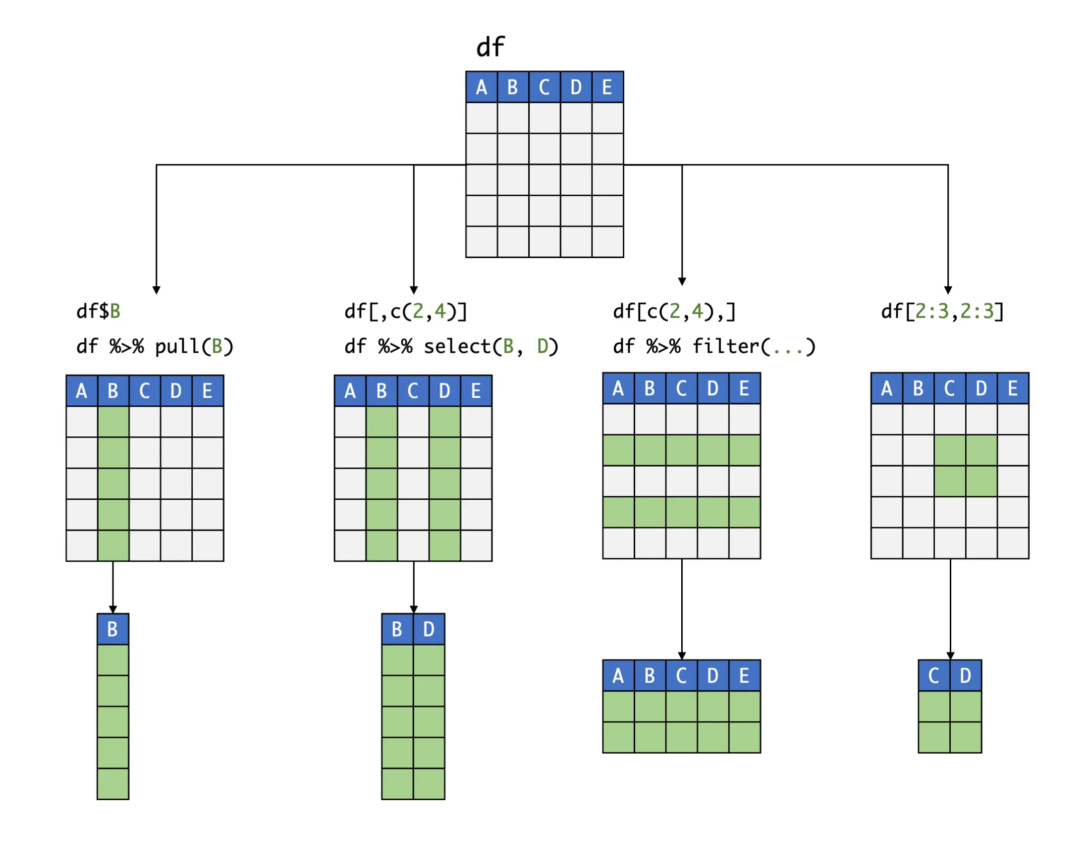
If one of the slots in the bracket (either the left or the right-hand side) is left empty, the entire row or column, respectively, is extracted:
data[,21]## [1] 0 0 1 0 0 1 1 1 0 1 0 0 0 1 0 1 0 1 1 1 1 0 1 1 1 1 0 0 [...]Instead of numbers, we can also use the name of a column as the index. Please note that, since rows typically do not have a name defined in the data frame, this is usually only possible for rows. To illustrate this, let us extract the first-row entry of the variable age:
data[1,"age"]## [1] 57Previously, we learned that relational operators can be used to determine if some condition (e.g. age > 40) is TRUE or FALSE. These resulting logical values can also be used as an index in the square brackets. Combining square brackets with relationship operators is particularly helpful because this allows filtering out data based on some pre-defined criteria. For example, if we want to extract the CES-D values of all individuals older than 40, we can use the following code:
data[data$age > 40,"cesd.0"]## [1] 24 35 36 28 34 42 38 27 37 27 25 20 37 21 17 26 28 32 [...]Slicing is also possible using the filter and select functions, which are part of the tidyverse. A special feature of these functions is that they are very “pipe-friendly”, which leads to less convoluted code when complex filters are applied. As an example, let us filter out all patients in data who are male (i.e. the variable sex equals 0) and older than 40, then select their CES-D values at all three assessment points, and then inspect the first three rows of the extracted data. That is a quite complex operation, but using a pipe makes it considerably easier to implement it:
data %>%
  filter(age > 40, sex == 0) %>%
  select(cesd.0, cesd.1, cesd.2) %>%
head(3)## cesd.0 cesd.1 cesd.2
## 1 37 13 5
## 2 27 31 38
## 3 25 33 6This concludes our brief journey into the R universe. Naturally, this brief overview is not enough to become a proficient R user, but the basics we covered here are a solid basis to proceed to the next chapter, in which we will begin with our hands-on analysis of RCT data. Before starting with the next chapter right away, it might be helpful to practice what we have learned in this part of the tutorial a little further. In the “Test Your Knowledge” box below, we have compiled a few coding exercises, with solutions provided at the end of the tutorial.
Especially for beginners, error messages and how to fix them tends to be one of the most excruciating parts of learning R. In GUI-based software, getting an error message usually means that something really, really bad has happened, so it is understandable that people tend to get nervous once the first red error messages start popping up. Thus, it is important to remember that everyone, even expert R programmers, get error messages all the time.
Deciphering and fixing error messages becomes easier with time, but even so, we have at our disposal one of the best troubleshooting tools thinkable: Google. If you get an error message that you find confusing, do not hesitate to copy and paste it into Google and search for results. There are countless programming forums on the Internet, and chances are high that someone was confronted with the same problem before. If your error message is not in English, it helps to set your locale to English first (using sys.setenv(LANG = "en"), because most programming content on the Internet is written in that language. If you run the code again, all messages should appear in English, and you are ready and set to search for help for them on the Internet.
Lastly, also make sure that your message is, in fact, an error message. R distinguishes between simple Messages, Warnings, and Errors. Only a message preceded by Error means that there was a fatal problem and that the code could not be run. Warnings alert us that something (may) have not worked as intended, but that the function could still be run. Messages work more like notes and tell us that some kind of operation or action has been performed for us by the function.
To complete the following exercises, our example RCT data set must be imported under the name data (see Section 1.3):
Log-transform the variable age in data and save the result as age.log.
Square all values in cesd.1 and save the result as cesd.1.squared within the data set data.
Calculate the mean and standard deviation (\(SD\)) of the variable cesd.2. If necessary, use the Internet to find out which function in R calculates the standard deviation of a numeric vector.
Save the calculated mean and standard deviation of cesd.2 in a list element.
Does the variable atsphs.0 in data have the desired class numeric? Try to confirm this using R code.
Create two new variables in data: (1) age.65plus, a logical variable which indicates if a person’s age is 65 or above; and (2) cesd.diff, a variable that contains the difference between cesd.0 and cesd.1 for each patient.
Using the pipe operator, filter out the records of all patients who are male (sex=0) and part of the intervention group (group=1); then, in this subset, select the variable age and calculate its mean.
In the fifth and sixth row of data, change the value of degree to NA (missing).
The solutions for these exercises are provided in the appendix.
\(\blacksquare\)
Since R version 4.1.0, a pipe operator is also available in Base R (meaning that no additional packages need to be loaded to use it). This Base R pipe works similarly to the tidyverse version that we will cover in this tutorial but uses the |> symbol instead. A detailed comparison of the tidyverse and Base R pipe is provided in this article.↩︎